Recognition: unknown
SHIFT: Robust Double Machine Learning for Average Dose-Response Functions under Heavy-Tailed Contamination
Pith reviewed 2026-05-09 20:14 UTC · model grok-4.3
The pith
SHIFT makes double machine learning for average dose-response functions robust to localized heavy-tailed contamination via a MAD-scaled defensive refit.
A machine-rendered reading of the paper's core claim, the machinery that carries it, and where it could break.
Core claim
SHIFT is a robust DML estimator for the average dose-response function that pairs nuisance orthogonalization with a Welsch loss optimized by graduated non-convexity and follows it with a defensive OLS refit whose inlier cutoff is scaled by the post-GNC residual MAD. This design achieves competitive worst-case shape recovery while recovering the ground-truth outlier mask at mean F1 approximately 0.96 on Gaussian-jump data generating processes.
What carries the argument
The defensive OLS refit with inlier cutoff scaled by post-GNC residual MAD, which self-calibrates the scale for tempering outliers in the second-stage kernel smoother.
If this is right
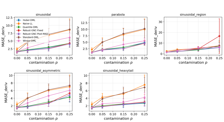
- Across 1400 fits, SHIFT shows competitive worst-case RMSE of 0.325 at p=0.25 for shape recovery.
- Among methods with worst-case RMSE below 0.35, only SHIFT provides non-uniform weights that recover the outlier mask at high F1.
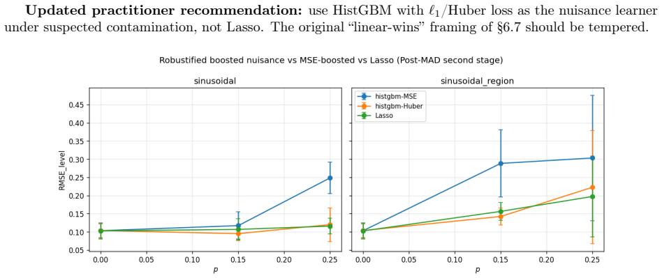
- Linear nuisance models such as Ridge and Lasso outperform gradient-boosted nuisances under uniform contamination.
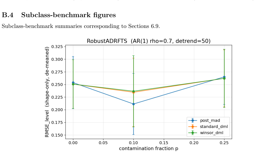
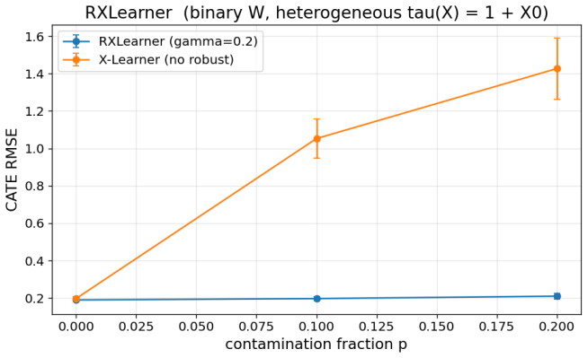
- Extensions include a Huber pseudo-outcome X-Learner for binary-treatment CATE and block cross-validation with rolling MAD for time-series ADRF.
- The EVT suite allows distinguishing Frechet from Weibull regimes to choose SHIFT or L1 alternatives.
Where Pith is reading between the lines
- The finding that linear nuisances are preferable under contamination inverts the usual preference for flexible models and may indicate that flexibility increases sensitivity to outliers even after robustification.
- Recovering the outlier mask at high accuracy allows SHIFT to serve as a diagnostic tool for identifying which observations drive the contamination.
- The localized-contamination robustness may prove useful in applications where outliers arise from specific subpopulations or measurement errors in certain ranges of the dose.
- The diagnostic suite provides a practical way to select robust estimators based on empirical tail behavior rather than assuming a contamination model in advance.
Load-bearing premise
The post-GNC residual MAD provides a reliable scale for the inlier cutoff that correctly separates signal from contamination without introducing bias on clean or uniformly contaminated data.
What would settle it
A test on clean data where SHIFT's RMSE exceeds that of standard DML or where the MAD cutoff fails to identify inliers correctly on the Gaussian-jump data generating processes used in the paper.
Figures


read the original abstract
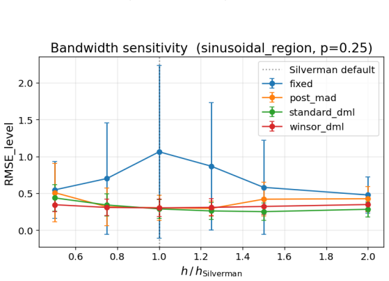
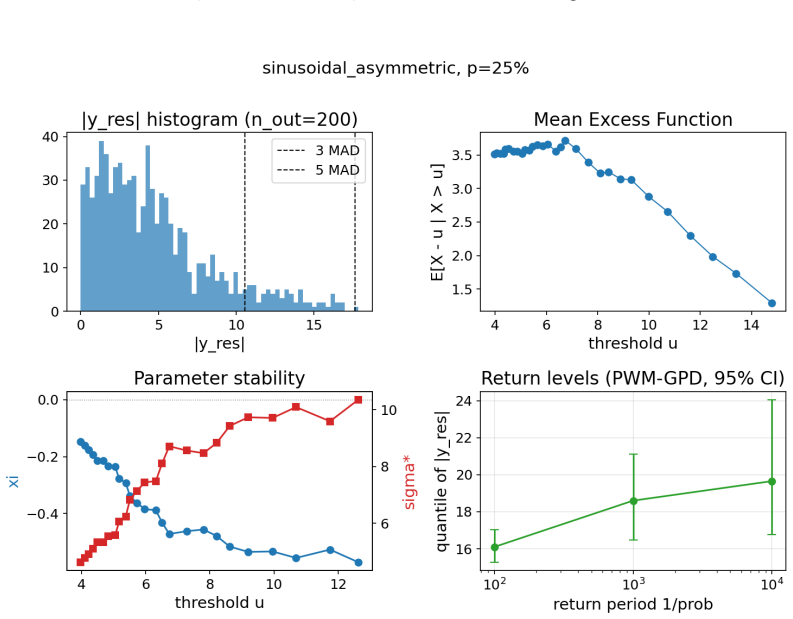
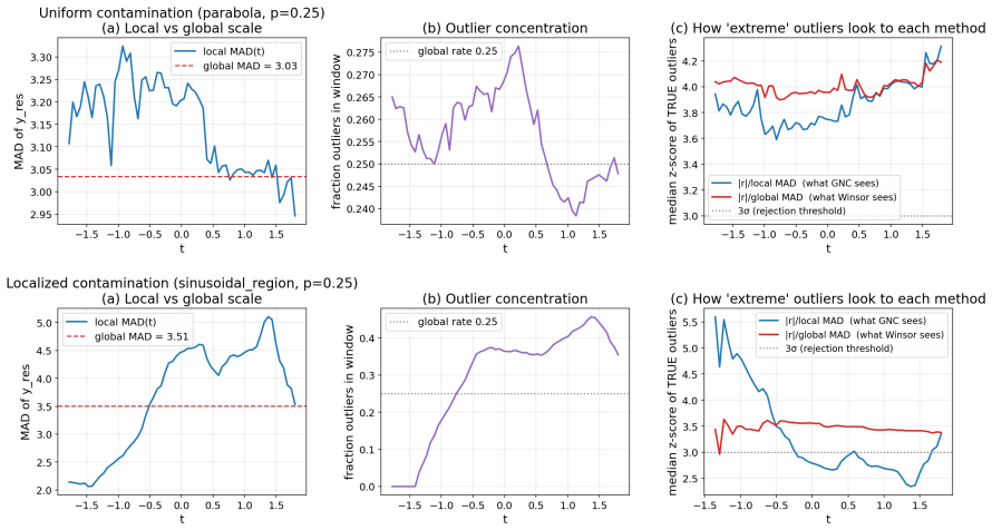
Double-machine-learning pipelines for the Average Dose-Response Function rely on kernel-weighted local-linear smoothers, which inherit unbounded functional influence: a single outlier within a kernel window biases the curve across the entire window. We introduce SHIFT (Self-calibrated Heavy-tail Inlier-Fit with Tempering), a robust DML estimator combining cross-fit nuisance orthogonalization with a kernel-local Welsch-loss second stage optimized by Graduated Non-Convexity, and -- the principal design choice -- a defensive OLS refit whose inlier cutoff is scaled by post-GNC residual MAD rather than the raw-outcome MAD. On a localized-contamination stress test at $p=0.25$ this design choice drops level-RMSE from 1.03 to 0.33 while leaving clean and uniformly-contaminated runs unchanged. Across 1,400 main-sweep fits, SHIFT has competitive worst-case shape recovery (RMSE $0.325$ at $p=0.25$, second to Huber-DML's $0.276$); among the three methods with worst-case RMSE below $0.35$, only SHIFT emits a non-uniform per-sample weight vector, recovering the ground-truth outlier mask at mean $F_1 \approx 0.96$ (range $0.945$--$0.968$) on Gaussian-jump DGPs. We pair the estimator with a six-technique Extreme Value Theory diagnostic suite (Hill, GPD-MLE/PWM, GEV, Mean Excess, parameter stability, causal tail coefficient) that lets a practitioner distinguish Frechet from Weibull regimes and choose between SHIFT and L1 alternatives on empirical grounds. Extensions to binary-treatment CATE (Huber pseudo-outcome X-Learner) and time-series ADRF (block-CV + rolling MAD) are included. A counter-intuitive ablation: linear nuisance models (Ridge, Lasso) outperform gradient-boosted nuisances for robust DML under uniform contamination, inverting the usual more-flexible-is-better heuristic.
Editorial analysis
A structured set of objections, weighed in public.
Referee Report
Summary. The manuscript presents SHIFT, a robust double machine learning estimator for average dose-response functions (ADRF) under heavy-tailed contamination. It integrates cross-fit nuisance orthogonalization with a kernel-local Welsch-loss second stage optimized using Graduated Non-Convexity (GNC), and features a defensive OLS refit where the inlier cutoff is scaled by the post-GNC residual median absolute deviation (MAD) rather than the raw MAD. Empirical results on localized-contamination stress tests at p=0.25 show a reduction in level-RMSE from 1.03 to 0.33, with competitive worst-case shape recovery (RMSE 0.325) across 1,400 fits and high outlier mask recovery (mean F1 ≈ 0.96). The paper also includes an Extreme Value Theory diagnostic suite for distinguishing contamination regimes and extensions to binary-treatment CATE and time-series ADRF, along with an ablation showing linear nuisance models outperforming gradient-boosted ones under uniform contamination.
Significance. If the reported performance improvements and the validity of the MAD scaling hold upon detailed verification, this work would represent a meaningful contribution to robust causal inference. It addresses the unbounded influence of outliers in kernel smoothers for ADRF estimation, provides a method that additionally recovers outlier masks, and offers diagnostics to guide method choice between SHIFT and alternatives like L1 or Huber. The counter-intuitive nuisance model finding could stimulate further research on model flexibility in robust settings.
major comments (2)
- [Abstract] The principal design choice of scaling the inlier cutoff by post-GNC residual MAD is credited with the RMSE improvement from 1.03 to 0.33 at localized p=0.25, but no separate diagnostic is provided to confirm that this MAD recovers the true inlier scale on clean data (p=0) or remains unbiased under uniform contamination, which is necessary to attribute the gain specifically to this choice rather than other components.
- [Empirical evaluation] The abstract reports specific RMSE values, F1 scores, and results from 1,400 main-sweep fits without mentioning error bars, standard deviations, or the full experimental protocol (including data-generating processes details beyond Gaussian-jump), and no mention of code availability, which undermines the ability to reproduce and assess the reliability of the claims.
minor comments (1)
- [Abstract] The abstract mentions 'six-technique Extreme Value Theory diagnostic suite (Hill, GPD-MLE/PWM, GEV, Mean Excess, parameter stability, causal tail coefficient)' but does not elaborate on how these are implemented or combined in the manuscript.
Simulated Author's Rebuttal
We thank the referee for their constructive comments and positive overall assessment of our work. We address each major comment below, indicating the revisions we will make to strengthen the manuscript.
read point-by-point responses
-
Referee: [Abstract] The principal design choice of scaling the inlier cutoff by post-GNC residual MAD is credited with the RMSE improvement from 1.03 to 0.33 at localized p=0.25, but no separate diagnostic is provided to confirm that this MAD recovers the true inlier scale on clean data (p=0) or remains unbiased under uniform contamination, which is necessary to attribute the gain specifically to this choice rather than other components.
Authors: We agree that an explicit diagnostic would better isolate the contribution of the MAD scaling. In the revised manuscript, we will add a new figure (or table in the appendix) that reports the estimated inlier scale (post-GNC residual MAD) versus the true inlier scale on clean data (p=0) and under uniform contamination across multiple replications. This will demonstrate that the scaling recovers the true scale without bias in those regimes, while still providing the robustness benefit under localized contamination. We will also clarify in the text that the unchanged performance on clean and uniform cases is consistent with unbiased scaling. revision: yes
-
Referee: [Empirical evaluation] The abstract reports specific RMSE values, F1 scores, and results from 1,400 main-sweep fits without mentioning error bars, standard deviations, or the full experimental protocol (including data-generating processes details beyond Gaussian-jump), and no mention of code availability, which undermines the ability to reproduce and assess the reliability of the claims.
Authors: We acknowledge the importance of reproducibility and statistical reliability. In the revision, we will: (1) include error bars or standard deviations for all reported metrics (e.g., RMSE, F1) based on the multiple replications; (2) expand the experimental protocol section with full details of all data-generating processes used, including parameters for the Gaussian-jump and other DGPs; (3) add a statement on code availability, with a link to a public repository containing the implementation and replication scripts. These changes will allow readers to fully assess and reproduce the results. revision: yes
Circularity Check
No significant circularity; estimator defined by explicit algorithmic choices with independent empirical validation
full rationale
The paper introduces SHIFT via a sequence of standard robust statistics components (cross-fit orthogonalization, Welsch loss with GNC optimization, post-GNC MAD-scaled defensive OLS refit) inside a DML pipeline for ADRF estimation. These are presented as design choices rather than derived quantities. Performance metrics (RMSE drops, F1 scores) are reported from Monte Carlo simulations on specified DGPs and are not obtained by refitting or renormalizing the same quantities used to define the estimator. No equations reduce a claimed prediction to its own fitted inputs by construction, no load-bearing self-citations appear, and no uniqueness theorem or ansatz is smuggled in. The derivation chain is therefore self-contained against external benchmarks.
Axiom & Free-Parameter Ledger
free parameters (2)
- inlier cutoff scale
- Welsch loss tuning parameter
axioms (2)
- domain assumption Standard double-machine-learning assumptions (unconfoundedness, overlap, correct nuisance estimation rates)
- domain assumption The contamination process admits a localized heavy-tailed component that the MAD-based cutoff can separate
Reference graph
Works this paper leans on
-
[1]
D. F. Andrews. A robust method for multiple linear regression.Technometrics, 16(4):523–531, 1974
1974
-
[2]
A. E. Beaton and J. W. Tukey. The fitting of power series, meaning polynomials, illustrated on band-spectroscopic data.Technometrics, 16(2):147–185, 1974
1974
-
[3]
Beirlant, Y
J. Beirlant, Y. Goegebeur, J. Segers, and J. Teugels.Statistics of Extremes: Theory and Applications. Wiley, 2004
2004
-
[4]
Bergmeir and J
C. Bergmeir and J. M. Benítez. On the use of cross-validation for time series predictor evaluation. Information Sciences, 191:192–213, 2012
2012
-
[5]
Blake and A
A. Blake and A. Zisserman.Visual Reconstruction. MIT Press, 1987
1987
-
[6]
Bonvini and E
M. Bonvini and E. H. Kennedy. Sensitivity analysis via the proportion of unmeasured confounding. Journal of the American Statistical Association, 2022
2022
-
[7]
H. Chen, T. Harinen, J.-Y. Lee, M. Yung, and Z. Zhao. CausalML: Python package for causal machine learning.https://github.com/uber/causalml, 2020
2020
-
[8]
Cheng, J
M.-Y. Cheng, J. Fan, and J. S. Marron. On boundary correction for local polynomial regression.Annals of Statistics, 25(4):1691–1708, 1997
1997
-
[9]
Chernozhukov, D
V. Chernozhukov, D. Chetverikov, M. Demirer, E. Duflo, C. Hansen, W. Newey, and J. Robins. Double/debiased machine learning for treatment and structural parameters.The Econometrics Journal, 21(1):C1–C68, 2018
2018
-
[10]
V. Chernozhukov, W. K. Newey, V. Quintas-Martinez, and V. Syrgkanis. Automatic debiased machine learning via riesz regression.arXiv preprint arXiv:2402.01785, 2024
-
[11]
W. S. Cleveland and S. J. Devlin. Locally weighted regression: an approach to regression analysis by local fitting.Journal of the American Statistical Association, 83(403):596–610, 1988. 31
1988
-
[12]
K. Colangelo and Y.-Y. Lee. Double debiased machine learning nonparametric inference with continuous treatments.arXiv preprint arXiv:2004.03036, 2020
-
[13]
Coles.An Introduction to Statistical Modeling of Extreme Values
S. Coles.An Introduction to Statistical Modeling of Extreme Values. Springer, 2001
2001
-
[14]
Dettling and P
M. Dettling and P. Bühlmann. Boosting for tumor classification with gene expression data.Bioinformatics, 19(9):1061–1069, 2003
2003
-
[15]
J. Dorn, D. Small, and K. Guo. Robust IV inference in heavy-tailed settings.arXiv preprint, 2024
2024
-
[16]
Dukes, T
O. Dukes, T. Martinussen, and E. J. Tchetgen Tchetgen. On robust inference in the nonparametric causal-inference setting with continuous exposures.arXiv preprint, 2024
2024
-
[17]
B. Efron. Better bootstrap confidence intervals.Journal of the American Statistical Association, 82(397): 171–185, 1987
1987
-
[18]
Fan and I
J. Fan and I. Gijbels.Local Polynomial Modelling and Its Applications. Chapman & Hall, 1996
1996
-
[19]
Fujisawa and S
H. Fujisawa and S. Eguchi. Robust parameter estimation with a small bias against heavy contamination. Journal of Multivariate Analysis, 99(9):2053–2081, 2008
2053
-
[20]
Gnecco, N
N. Gnecco, N. Meinshausen, J. Peters, and S. Engelke. Causal discovery in heavy-tailed models.Annals of Statistics, 49(3):1755–1778, 2021
2021
-
[21]
F. R. Hampel, E. M. Ronchetti, P. J. Rousseeuw, and W. A. Stahel.Robust Statistics: The Approach Based on Influence Functions. Wiley, 1986
1986
-
[22]
B. M. Hill. A simple general approach to inference about the tail of a distribution.Annals of Statistics, 3(5):1163–1174, 1975
1975
-
[23]
P. J. Huber.Robust Statistics. Wiley, 1981
1981
-
[24]
Y. Jin, Z. Ren, and E. J. Candès. Wasserstein sensitivity of observational studies: distributionally robust causal effects.Journal of the American Statistical Association, 2023
2023
-
[25]
Kallus, X
N. Kallus, X. Mao, and M. Uehara. Robust heterogeneous treatment effects under contamination.arXiv preprint, 2024
2024
-
[26]
Kanamori and M
T. Kanamori and M. Sugiyama. Robust estimation via robust gradient estimation.Bernoulli, 2015
2015
-
[27]
E. H. Kennedy. Towards optimal doubly robust estimation of heterogeneous causal effects.Electronic Journal of Statistics, 17(2):3008–3049, 2023
2023
-
[28]
Koenker.Quantile Regression
R. Koenker.Quantile Regression. Cambridge University Press, 2005
2005
-
[29]
S. R. Künzel, J. S. Sekhon, P. J. Bickel, and B. Yu. Metalearners for estimating heterogeneous treatment effects using machine learning.Proceedings of the National Academy of Sciences, 116(10):4156–4165, 2019
2019
-
[30]
Le, T.-J
H. Le, T.-J. Chin, and D. Suter. An exact penalty method for locally convergent maximum consensus. Computer Vision and Pattern Recognition (CVPR), 2017
2017
-
[31]
Y. G. Leclerc. Constructing simple stable descriptions for image partitioning.International Journal of Computer Vision, 3(1):73–102, 1989
1989
-
[32]
R. A. Maronna, R. D. Martin, V. J. Yohai, and M. Salibián-Barrera.Robust Statistics: Theory and Methods (with R). Wiley, 2nd edition, 2019
2019
-
[33]
EconML: A python package for ML-based heterogeneous treatment effects estimation
Microsoft Research. EconML: A python package for ML-based heterogeneous treatment effects estimation. https://github.com/py-why/EconML, 2019. 32
2019
-
[34]
Mobahi and J
H. Mobahi and J. W. Fisher III. On the link between Gaussian homotopy continuation and convex envelopes. InEnergy Minimization Methods in Computer Vision and Pattern Recognition, 2015
2015
-
[35]
L. Nie, M. Ye, Q. Liu, and D. Nicolae. VCNet and functional targeted regularization for learning causal effects of continuous treatments. InInternational Conference on Learning Representations, 2021
2021
-
[36]
Nie and S
X. Nie and S. Wager. Quasi-oracle estimation of heterogeneous treatment effects.Biometrika, 108(2): 299–319, 2021
2021
-
[37]
Pedregosa, G
F. Pedregosa, G. Varoquaux, A. Gramfort, V. Michel, B. Thirion, O. Grisel, M. Blondel, P. Prettenhofer, R. Weiss, V. Dubourg, et al. Scikit-learn: Machine learning in Python.Journal of Machine Learning Research, 12:2825–2830, 2011
2011
-
[38]
J. Racine. Consistent cross-validatory model-selection for dependent data: hv-block cross-validation. Journal of Econometrics, 99(1):39–61, 2000
2000
-
[39]
P. J. Rousseeuw and A. M. Leroy.Robust Regression and Outlier Detection. Wiley, 1987
1987
-
[40]
Semenova and V
V. Semenova and V. Chernozhukov. Debiased machine learning of conditional average treatment effects and other causal functions.The Econometrics Journal, 24(2):264–289, 2021
2021
-
[41]
Tübbicke
S. Tübbicke. Entropy balancing for continuous treatments.Journal of Econometric Methods, 2022
2022
-
[42]
M. J. van der Laan, J. R. Coyle, H. Rytgaard, and W. Cai. Higher-order targeted minimum loss-based estimation with the highly adaptive lasso.arXiv preprint, 2024
2024
-
[43]
S. Wager. Causal inference under heavy-tailed responses.Statistical Science, 2024
2024
-
[44]
H. Yang, P. Antonante, V. Tzoumas, and L. Carlone. Graduated non-convexity for robust spatial perception: From non-minimal solvers to global outlier rejection.IEEE Robotics and Automation Letters, 5(2):1127–1134, 2020
2020
-
[45]
H. Yang, J. Shi, and L. Carlone. TEASER: Fast and certifiable point cloud registration.IEEE Transactions on Robotics, 37(2):314–333, 2021
2021
-
[46]
V. J. Yohai. High breakdown-point and high efficiency robust estimates for regression.Annals of Statistics, 15(2):642–656, 1987
1987
-
[47]
W. Zhou and R. Song. Doubly robust estimation of causal effects under heavy-tailed errors.arXiv preprint arXiv:2404.09148, 2024. A Thematic appendix index and FAQ cross-reference The appendices span∼ 30pages across A–K and address a wide range of anticipated reader questions in depth (per-cell statistics, sensitivity sweeps, ablations, theory, baselines, ...
-
[48]
Rank-indistinguishable tail.Student- tν with ν≤ 3and small-magnitude contamination: F1 plateaus
-
[49]
In our main sweep, p≤0.25, so this is out of scope but worth flagging for deployment
Asymmetric + p > 0.3.A one-sided mean shift with> 30%contamination pushes the robust estimators’ median-based initial estimate off the structural trend, and GNC cannot recover. In our main sweep, p≤0.25, so this is out of scope but worth flagging for deployment. D.8 A practitioner workflow We suggest the following:
-
[50]
Inspect the per-sample weight vector for a candidate outlier mask and the ADRF shape
RunSHIFTas the default. Inspect the per-sample weight vector for a candidate outlier mask and the ADRF shape
-
[51]
If Hill ˆα <3or GPD ˆξ > 0: switch toQuantile-DMLfor the point estimate; retainSHIFT’s mask for the detection report
Run the EVT diagnostic on theGNC-Fixedresiduals (or on(1−w r) ·r). If Hill ˆα <3or GPD ˆξ > 0: switch toQuantile-DMLfor the point estimate; retainSHIFT’s mask for the detection report
-
[52]
ConsiderHuber-DML for the point estimate;SHIFT’s mask can identify whichT-regions are affected
If the causal tail coefficientΓ(T→ |y res|) > 0.6: the contamination isT-dependent. ConsiderHuber-DML for the point estimate;SHIFT’s mask can identify whichT-regions are affected
-
[53]
51 This workflow gives the analyst defensible choice points rather than an opaque pipeline
If the percentile-bootstrap CI width is> 0.5· (signal scale), switch to BCa or studentized bootstrap, or use a block-wise resampling scheme if the data are dependent. 51 This workflow gives the analyst defensible choice points rather than an opaque pipeline. The tradeoff is human-in-the-loop effort; the payoff is that the final estimate is calibrated to t...
-
[54]
On localized contamination, slightly wider cutoffs win (less risk of rejecting inliers near the contaminated window)
The default3 σ is reasonable but not optimal for every DGP.On uniform-contamination sinusoidal, tighter cutoffs win (lower variance from rejecting more). On localized contamination, slightly wider cutoffs win (less risk of rejecting inliers near the contaminated window)
-
[55]
The post-GNC MAD source matters more than the cutoff multiplier
The architectural fix dominates the cutoff choice.Even at the worst cutoff (5.0 onsinusoidal), SHIFT’s RMSE is0.483, which is still better thanGNC-Fixed’s1.026at any cutoff (RMSE> 1at all of 2.0–5.0; data not shown). The post-GNC MAD source matters more than the cutoff multiplier
-
[56]
An EVT-informed adaptive cutoff is the natural next step.The current3σ targets a0 .27% Gaussian-tail exceedance rate. Replacing it with a GPD-fit-based threshold (parameter-stability or mean- excess diagnostics) would adapt to the actual tail shape and could close some of the0.05–0.10RMSE gap to the per-DGP optimum. EVT-calibrated cutoff: a concrete propo...
-
[57]
On the localized- contamination DGP it suffers the same failure mode asGNC-Fixed(RMSE > 1)
Post-GNC MAD differentiatesSHIFTfrom MM-LPR.MM-LPR-Tukey uses Tukey biweight (similar to Welsch) with MAD-scaled IRLS butwithoutthe post-fit residual MAD step. On the localized- contamination DGP it suffers the same failure mode asGNC-Fixed(RMSE > 1). This is positive evidence that the architectural fix matters beyond the choice of redescending loss
-
[58]
It loses toSHIFTon the localized-contamination cells
Robust-LOESS is competitive on uniform-Gaussian and on heavy-tail.The Cleveland-Devlin recipe (bisquare with iterated re-scaling at6 ·median|r| ) wins on sinusoidalp = 0 .25(0 .202) and sinusoidal_heavytailp = 0.15, 0.25(0 .124, 0.144). It loses toSHIFTon the localized-contamination cells. The two methods are complementary and a hybrid (Robust-LOESS for u...
-
[59]
We report the negative result
The hybrid Welsch + L1 idea does not help.The Welsch tail rejection is already aggressive; replacing the body fit with L1 instead of OLS on the inlier set adds variance without much bias reduction. We report the negative result
-
[60]
alignment to the grid-mean of intercepts is ad hoc
Trimmed-LL is biased downward.As in our earlier Trimmed-DML result (App. D), simple top-/bottom- residual trimming changes the estimand and produces0.10–0.30extra RMSE on uniform contamination. Figure 35: Robust local-polynomial baselines on three DGPs. 64 H.2 ADRF integration anchoring schemes The defaultSHIFTanchors the integration constant by aligning ...
-
[61]
Warm starts across neighboring grid points.The IRLS solution att0 is a strong initial guess for t0 + ∆t; this would reduceJfrom≈5to≈2on contiguous grid points
-
[62]
Cached kernel sums.The kernel weightsKh( ˜Ti −t 0)are translation-invariant in t0; for evenly-spaced grids, an FFT-based convolution computes allGkernel sums inO(nlogG)
-
[63]
Parallel grid evaluation.Trivially exploitable since eacht0 is independent. Our reference is single- threaded for reproducibility but ajoblib.Parallelwrapper drops total time linearly with cores. J.4 EVT on weight-induced ranking one might ask whether using the final weight ordering (rather than GNC-Fixed residuals) would change tail inferences. We have i...
-
[64]
Cross-cutoff Jaccard:for the same seed and DGP,| ˆMc1 ∩ ˆMc2 |/| ˆMc1 ∪ ˆMc2 | where ˆMc is the bottom-c- fraction-by-weight mask
-
[65]
Mask-vs-truth Jaccard: | ˆMc ∩M ⋆|/| ˆMc ∪M ⋆| where M ⋆ is the ground-truth contamination mask from the DGP
-
[66]
Cross-seed rank-correlation RMS:for the same DGP across seeds, root-mean-square distance between rank-percentiles of the weight vector. 73 DGP/ cutoff fraction 0.05 0.10 0.15 0.20 Mask-vs-ground-truth Jaccard (true contaminationp= 0.25): sinusoidal0.200 0.400 0.6000.800 sinusoidal_region0.200 0.400 0.6000.796 sinusoidal_heavytail0.196 0.380 0.5030.537 Cro...
discussion (0)
Sign in with ORCID, Apple, or X to comment. Anyone can read and Pith papers without signing in.