Recognition: unknown
Adaptive anisotropic composite quadratures for residual minimisation in neural PDE approximations
Pith reviewed 2026-05-09 19:32 UTC · model grok-4.3
The pith
An adaptive quadrature method controls integration errors to improve neural network solutions of PDEs obtained by residual minimization.
A machine-rendered reading of the paper's core claim, the machinery that carries it, and where it could break.
Core claim
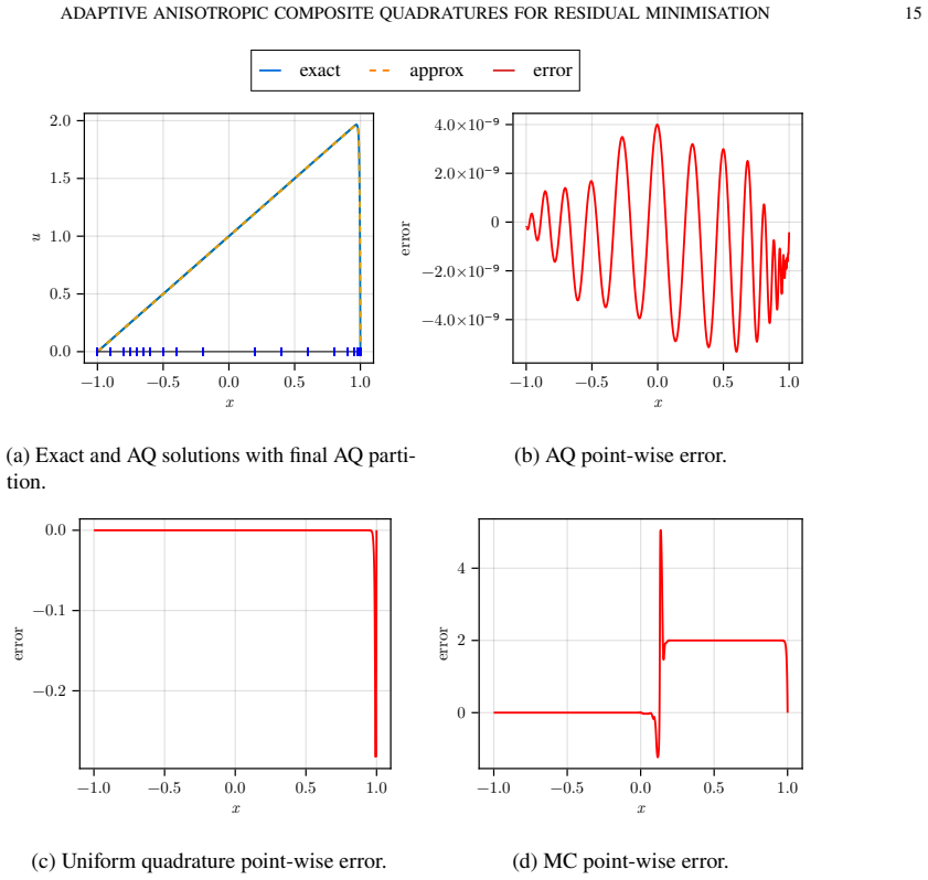
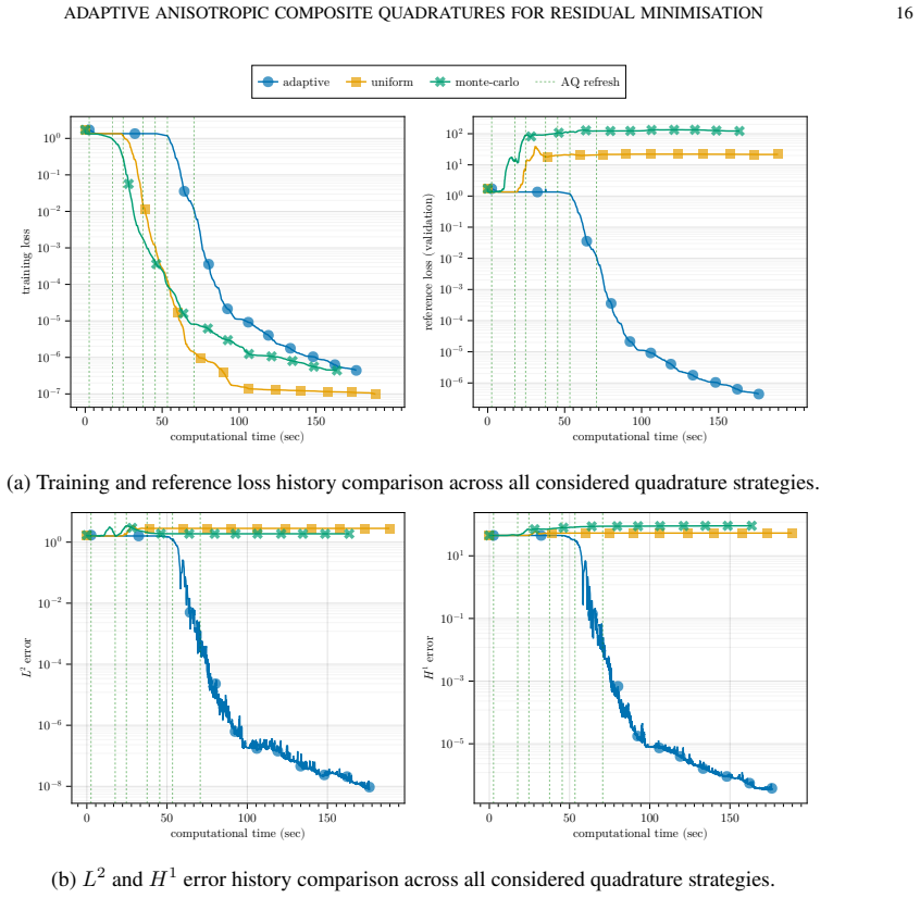
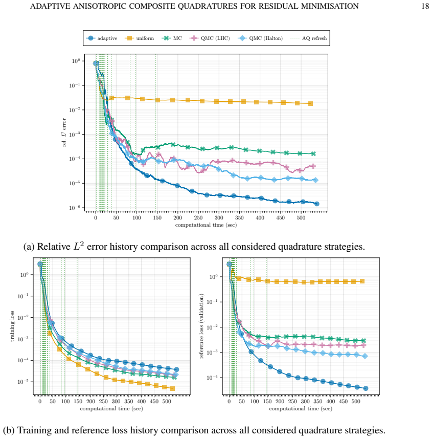
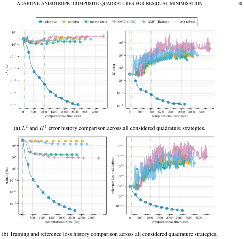
By separating approximation, quadrature and optimization errors in an abstract framework and deriving a nonlinear Strang-type estimate, the authors justify an anisotropic adaptive composite quadrature that controls relative quadrature error through richer reference rules and bisection refinement; this is paired with a refresh-based training procedure that rebuilds the quadrature only when an online error indicator exceeds a threshold. Numerical tests on benchmark PDEs show that the resulting training loss stays closer to the reference loss, quadrature points are used more efficiently, and final approximation accuracy exceeds that of non-adaptive strategies.
What carries the argument
The anisotropic adaptive composite quadrature strategy, which uses bisection-based refinement against richer reference quadratures to keep relative quadrature error of the residual loss below a threshold, combined with a refresh-based training loop triggered by an online error indicator.
If this is right
- The gap between the training loss and a reference loss computed with very fine quadrature narrows.
- Quadrature points are allocated more efficiently than with fixed non-adaptive rules.
- Final neural approximations achieve higher accuracy than those obtained with non-adaptive quadrature strategies.
- Computational cost is balanced by rebuilding the quadrature only when the online indicator signals that error has grown too large.
Where Pith is reading between the lines
- The same refresh-based logic could be applied to other loss functions that rely on numerical integration, such as energy minimization or variational formulations.
- The abstract error framework offers a template for analyzing Monte Carlo or low-discrepancy sampling errors in neural PDE solvers.
- Because the refinement is anisotropic, the method may naturally extend to problems with strong directional features such as boundary layers or anisotropic coefficients.
Load-bearing premise
The abstract error framework and derived nonlinear Strang-type estimate correctly quantify how quadrature inaccuracies affect the final neural approximation, and the online error indicator reliably detects when quadrature error becomes significant.
What would settle it
A benchmark PDE test in which the adaptive method leaves a large persistent gap between training loss and a reference loss computed on a much finer quadrature, or in which the online indicator fails to trigger refinement in subdomains where the residual is known to be large.
Figures


read the original abstract
We study the role of numerical quadrature in residual-minimisation methods for neural network approximation of partial differential equations. We first present an abstract error framework that separates approximation, quadrature and optimisation errors, and derive a nonlinear Strang-type estimate quantifying how inaccuracies in the discrete loss affect the final approximation. Motivated by this analysis, we propose an anisotropic adaptive composite quadrature strategy that controls the relative quadrature error of the residual loss using richer reference quadratures and bisection-based refinement. We then introduce a refresh-based training methodology that rebuilds the quadrature only when an online error indicator exceeds a prescribed threshold, balancing accuracy and computational cost. Numerical experiments on a range of benchmark problems show that the proposed approach narrows the gap between training and reference losses, uses quadrature points more efficiently and delivers strong approximation accuracy relative to non-adaptive quadrature strategies.
Editorial analysis
A structured set of objections, weighed in public.
Referee Report
Summary. The paper presents an abstract error framework separating approximation, quadrature, and optimization errors in residual-minimization methods for neural network approximations of PDEs. It derives a nonlinear Strang-type estimate to quantify the effect of quadrature inaccuracies on the final approximation. Motivated by this, the authors propose an anisotropic adaptive composite quadrature strategy using richer reference quadratures and bisection-based refinement to control relative quadrature error, along with a refresh-based training methodology that rebuilds the quadrature only when an online error indicator exceeds a threshold. Numerical experiments on benchmark problems claim that the approach narrows the gap between training and reference losses, uses quadrature points more efficiently, and achieves strong approximation accuracy relative to non-adaptive strategies.
Significance. If the error framework and Strang-type estimate hold under the conditions of the method, and the adaptive strategy reliably detects and controls quadrature error, this could be a meaningful contribution to improving the reliability and efficiency of neural PDE solvers. The refresh mechanism offers a practical way to balance cost and accuracy, and the experimental results on benchmarks suggest potential for broader adoption if the improvements prove robust beyond the tested cases.
major comments (2)
- [§3] §3 (nonlinear Strang-type estimate): The central claim that the estimate quantifies how quadrature inaccuracies affect the neural approximation depends on assumptions (e.g., Lipschitz continuity or local convexity of the loss) that are not explicitly verified for the non-convex residual losses typical in PINN training. The derivation should state these assumptions clearly and include a check or counterexample showing when they hold or fail, as this underpins the motivation for the adaptive quadrature.
- [§5] §5 (numerical experiments): The reported improvements in narrowing the train-reference loss gap and efficient quadrature use rely on the online error indicator correlating with actual approximation degradation. The manuscript should provide more detail on how the reference quadratures are constructed, the number of independent runs, and statistical measures of improvement to confirm the gains are not problem-specific or due to particular hyperparameter choices.
minor comments (3)
- [§4] The notation for the anisotropic composite quadrature and the error indicator in §4 could be clarified, perhaps with a pseudocode algorithm or diagram showing the bisection refinement process.
- [Introduction] A few sentences in the introduction could better distinguish the proposed method from prior adaptive quadrature techniques in finite elements or other neural PDE papers to highlight novelty.
- [§5] Figure captions for the benchmark results should explicitly state the quadrature point counts and loss values for both adaptive and non-adaptive cases to aid direct comparison.
Simulated Author's Rebuttal
We thank the referee for the constructive report and positive assessment of the potential contribution. We address each major comment below and will incorporate the indicated revisions in the next version of the manuscript.
read point-by-point responses
-
Referee: [§3] §3 (nonlinear Strang-type estimate): The central claim that the estimate quantifies how quadrature inaccuracies affect the neural approximation depends on assumptions (e.g., Lipschitz continuity or local convexity of the loss) that are not explicitly verified for the non-convex residual losses typical in PINN training. The derivation should state these assumptions clearly and include a check or counterexample showing when they hold or fail, as this underpins the motivation for the adaptive quadrature.
Authors: We agree that the assumptions should be stated more explicitly. The nonlinear Strang-type estimate is derived in an abstract setting under the hypothesis that the loss is locally Lipschitz continuous with respect to quadrature perturbations; this is satisfied for smooth residuals but need not hold globally for non-convex PINN losses. We will revise §3 to list the assumptions explicitly and add a short discussion of their local validity near approximate minima, where the loss behaves more convexly. A full counterexample lies outside the scope of the abstract framework, but we will note the conditions under which the bound may become loose. revision: yes
-
Referee: [§5] §5 (numerical experiments): The reported improvements in narrowing the train-reference loss gap and efficient quadrature use rely on the online error indicator correlating with actual approximation degradation. The manuscript should provide more detail on how the reference quadratures are constructed, the number of independent runs, and statistical measures of improvement to confirm the gains are not problem-specific or due to particular hyperparameter choices.
Authors: We will expand the experimental section to describe the reference quadratures in detail (high-order adaptive tensor-product Gauss-Legendre rules with bisection refinement), report all metrics as averages over 10 independent runs with distinct random seeds, and include means together with standard deviations for the training-reference loss gaps and approximation errors. These additions will demonstrate that the observed improvements are robust across initializations and not tied to specific hyperparameter choices. revision: yes
Circularity Check
No significant circularity in derivation chain
full rationale
The paper first presents an abstract error framework that separates approximation, quadrature, and optimisation errors, then derives a nonlinear Strang-type estimate from it. This analysis is positioned as independent motivation for the proposed adaptive composite quadrature and refresh-based training. The numerical experiments validate the approach on external benchmark problems rather than using fitted outcomes to define or predict the method itself. No self-citations are invoked as load-bearing uniqueness theorems, no ansatz is smuggled via prior work, and no known result is merely renamed. The derivation remains self-contained against the stated benchmarks and error analysis.
Axiom & Free-Parameter Ledger
axioms (1)
- domain assumption Abstract error framework that separates approximation, quadrature, and optimisation errors
Reference graph
Works this paper leans on
-
[1]
Interpolation error estimates inW 1,p for degenerateQ1 isoparametric elements
G. Acosta and G. Monzón. “Interpolation error estimates inW 1,p for degenerateQ1 isoparametric elements”. In:Numerische Mathematik, 104.2 (2006), pp. 129–150.doi:10.1007/s00211-006- 0018-1
-
[2]
Learning in PINNs: Phasetransition,diffusionequilibrium,andgeneralization
S. J. Anagnostopoulos, J. D. Toscano, N. Stergiopulos, and G. E. Karniadakis. “Learning in PINNs: Phasetransition,diffusionequilibrium,andgeneralization”.In:NeuralNetworks,193,107983(2026). doi:https://doi.org/10.1016/j.neunet.2025.107983
-
[3]
Numerical Experience with a Class of Self-Scaling Quasi-Newton Algorithms
M. Al-Baali. “Numerical Experience with a Class of Self-Scaling Quasi-Newton Algorithms”. In:Journal of Optimization Theory and Applications(1998), pp. 533–553.doi: 10 . 1023 / A : 1022608410710
1998
-
[4]
S. Badia, W. Li, and A. F. Martín. “Adaptive finite element interpolated neural networks”. In: Computer Methods in Applied Mechanics and Engineering, 437, 117806 (2025).doi:https : //doi.org/10.1016/j.cma.2025.117806
-
[5]
Compatible finite element interpolated neural networks
S. Badia, W. Li, and A. F. Martín. “Compatible finite element interpolated neural networks”. In: Computer Methods in Applied Mechanics and Engineering, 439, 117889 (2025).doi:https : //doi.org/10.1016/j.cma.2025.117889
-
[6]
S. Badia and F. Verdugo. “Gridap: An extensible Finite Element toolbox in Julia”. In:Journal of Open Source Software, 5.52, 2520 (2020).doi:10.21105/joss.02520
-
[7]
S. Berrone, C. Canuto, and M. Pintore. “Variational Physics Informed Neural Networks: the Role of Quadratures and Test Functions”. In:Journal of Scientific Computing, 92.3, 100 (2022).doi: 10.1007/s10915-022-01950-4
-
[8]
Effective Extensible Programming: Unleashing Julia on GPUs
T. Besard, C. Foket, and B. De Sutter. “Effective Extensible Programming: Unleashing Julia on GPUs”. In:IEEE Transactions on Parallel and Distributed Systems(2018).doi:10.1109/TPDS. 2018.2872064. arXiv:1712.03112 [cs.PL]
-
[9]
J. Bezanson, A. Edelman, S. Karpinski, and V. B. Shah. “Julia: A Fresh Approach to Numerical Computing”. In:SIAM Review, 59.1 (2017), pp. 65–98.doi:10.1137/141000671
-
[10]
Z. Cai, J. Chen, M. Liu, and X. Liu. “Deep least-squares methods: An unsupervised learning-based numerical method for solving elliptic PDEs”. In:Journal of Computational Physics, 420, 109707 (2020).doi:https://doi.org/10.1016/j.jcp.2020.109707
-
[11]
Makie.jl: Flexible high-performance data visualization for Julia
S. Danisch and J. Krumbiegel. “Makie.jl: Flexible high-performance data visualization for Julia”. In: Journal of Open Source Software, 6.65 (2021), p. 3349.doi:10.21105/joss.03349
-
[12]
T.DeRyck,S.Lanthaler,andS.Mishra.“Ontheapproximationoffunctionsbytanhneuralnetworks”. In:Neural Networks, 143 (2021), pp. 732–750.doi:https://doi.org/10.1016/j.neunet. 2021.08.015
-
[13]
Neural-network-based approximations for solving partial differential equations
M. Dissanayake and N. Phan-Thien. “Neural-network-based approximations for solving partial differential equations”. In:Communications in Numerical Methods in Engineering, 10.3 (1994), pp. 195–201.doi:https://doi.org/10.1002/cnm.1640100303. REFERENCES 34
-
[14]
A. Ern and J.-L. Guermond.Finite Elements II. 1st ed. Springer Cham, 2021.doi:https://doi. org/10.1007/978-3-030-56923-5
-
[15]
Computational Math with Neural Networks is Hard
M. Feischl and F. Zehetgruber. “Computational Math with Neural Networks is Hard”. In:arXiv pre-printrepository(2025).Referredpre-printversion- [v1].arXiv: 2505.17751 [math.NA].url: https://arxiv.org/abs/2505.17751
-
[16]
A. Genz and A. Malik. “Remarks on algorithm 006: An adaptive algorithm for numerical integration over an N-dimensional rectangular region”. In:Journal of Computational and Applied Mathematics, 6.4 (1980), pp. 295–302.doi:https://doi.org/10.1016/0771-050X(80)90039-X
-
[17]
An adaptive numerical integration algorithm for simplices
A. Genz. “An adaptive numerical integration algorithm for simplices”. In:Computing in the 90’s. Ed. by N. A. Sherwani, E. de Doncker, and J. A. Kapenga. New York, NY: Springer New York, 1991, pp. 279–285.url:https://doi.org/10.1007/BFb0038504
-
[18]
An adaptive numerical cubature algorithm for simplices
A. Genz and R. Cools. “An adaptive numerical cubature algorithm for simplices”. In:ACM Trans. Math. Softw., 29.3 (2003), pp. 297–308.doi:10.1145/838250.838254
-
[19]
High-Re solutions for incompressible flow using the Navier-Stokes equations and a multigrid method
U. Ghia, K. Ghia, and C. Shin. “High-Re solutions for incompressible flow using the Navier-Stokes equations and a multigrid method”. In:Journal of Computational Physics, 48.3 (1982), pp. 387–411. doi:https://doi.org/10.1016/0021-9991(82)90058-4
-
[20]
Understandingthedifficultyoftrainingdeepfeedforwardneuralnetworks
X.GlorotandY.Bengio.“Understandingthedifficultyoftrainingdeepfeedforwardneuralnetworks”. In:Proceedings of the Thirteenth International Conference on Artificial Intelligence and Statistics. Ed. by Y. W. Teh and M. Titterington. Vol. 9. Proceedings of Machine Learning Research. Chia Laguna Resort, Sardinia, Italy: PMLR, 2010, pp. 249–256.url:https://procee...
2010
-
[21]
AFiniteElementTechniqueforSolvingFirst-OrderPDEsin Lp
J.L.Guermond.“AFiniteElementTechniqueforSolvingFirst-OrderPDEsin Lp”.In:SIAMJournal on Numerical Analysis, 42.2 (2004), pp. 714–737.doi:10.1137/S0036142902417054
-
[22]
Algorithm 851: CG_DESCENT, a conjugate gradient method with guaranteed descent
W. W. Hager and H. Zhang. “Algorithm 851: CG_DESCENT, a conjugate gradient method with guaranteed descent”. In:ACM Trans. Math. Softw., 32.1 (2006), pp. 113–137.doi:10 . 1145 / 1132973.1132979
-
[23]
Don’tUnrollAdjoint:DifferentiatingSSA-FormPrograms
M.Innes.“Don’tUnrollAdjoint:DifferentiatingSSA-FormPrograms”.In:arXivpre-printrepository (2019). Referred pre-print version -[v4].url: https://doi.org/10.48550/arXiv.1810. 07951
-
[24]
Flux: Elegant machine learning with Julia
M. Innes. “Flux: Elegant machine learning with Julia”. In:Journal of Open Source Software, 3.25, 602 (2018).doi:10.21105/joss.00602
-
[25]
S. G. Johnson.The HCubature.jl package for multi-dimensional adaptive integration in Julia. https://github.com/JuliaMath/HCubature.jl. 2017
2017
-
[26]
E. Kiyani, K. Shukla, J. F. Urbán, J. Darbon, and G. E. Karniadakis. “Optimizing the optimizer for physics-informed neural networks and Kolmogorov-Arnold networks”. In:Computer Methods in Applied Mechanics and Engineering, 446, 118308 (2025).doi:https://doi.org/10.1016/j. cma.2025.118308
work page doi:10.1016/j 2025
-
[27]
In: Advances in Neural Information Processing Systems, vol
A.S.Krishnapriyan,A.Gholami,S.Zhe,R.M.Kirby,andM.W.Mahoney.“Characterizingpossible failure modes in physics-informed neural networks”. In:arXiv pre-print repository(2021). Referred pre-print version -[v2].url:https://doi.org/10.48550/arXiv.2109.01050
-
[28]
IEEE Transactions on Neural Networks 9(5), 987–1000 (1998) https://doi.org/10.1109/72.712178
I. Lagaris, A. Likas, and D. Fotiadis. “Artificial neural networks for solving ordinary and partial differential equations”. In:IEEE Transactions on Neural Networks, 9.5 (1998), pp. 987–1000.doi: 10.1109/72.712178
-
[29]
Fourier Neural Operator for Parametric Partial Differential Equations
Z.Lietal.“FourierNeuralOperatorforParametricPartialDifferentialEquations”.In:arXivpre-print repository(2021).Referredpre-printversion- [v3].url: https://arxiv.org/abs/2010.08895
work page internal anchor Pith review arXiv 2021
-
[30]
Adaptive two-layer ReLU neural network: I. Best least-squares approximation
M. Liu, Z. Cai, and J. Chen. “Adaptive two-layer ReLU neural network: I. Best least-squares approximation”. In:Computers & Mathematics with Applications, 113 (2022), pp. 34–44.doi: https://doi.org/10.1016/j.camwa.2022.03.005
-
[31]
Deep Ritz method with adaptive quadrature for linear elasticity
M. Liu, Z. Cai, and K. Ramani. “Deep Ritz method with adaptive quadrature for linear elasticity”. In:Computer Methods in Applied Mechanics and Engineering, 415, 116229 (2023).doi:https: //doi.org/10.1016/j.cma.2023.116229
-
[32]
LearningnonlinearoperatorsviaDeepONet based on the universal approximation theorem of operators
L.Lu,P.Jin,G.Pang,Z.Zhang,andG.E.Karniadakis.“LearningnonlinearoperatorsviaDeepONet based on the universal approximation theorem of operators”. In:Nature Machine Intelligence, 3.3 (2021), pp. 218–229. REFERENCES 35
2021
-
[33]
A. Magueresse and S. Badia. “Adaptive quadratures for nonlinear approximation of low-dimensional PDEs using smooth neural networks”. In:Computers & Mathematics with Applications, 162 (2024), pp. 1–21.doi:https://doi.org/10.1016/j.camwa.2024.02.041
-
[34]
W. F. Mitchell.NIST Adaptive Mesh Refinement (AMR) Benchmark Problems. Last updated March 6,
-
[35]
2013.url:https://math.nist
National Institute of Standards and Technology (NIST). 2013.url:https://math.nist. gov/amr-benchmark/index.html(visited on 12/22/2025)
2013
-
[36]
Optim: A mathematical optimization package for Julia
P. K. Mogensen and A. N. Riseth. “Optim: A mathematical optimization package for Julia”. In: Journal of Open Source Software, 3.24, 615 (2018).doi:10.21105/joss.00615
-
[37]
W. J. Morokoff and R. E. Caflisch. “Quasi-Monte Carlo Integration”. In:Journal of Computational Physics, 122.2 (1995), pp. 218–230.doi:https://doi.org/10.1006/jcph.1995.1209
-
[38]
Physics-informed neural networks: A deep learning frameworkforsolvingforwardandinverseproblemsinvolvingnonlinearpartialdifferentialequations
M. Raissi, P. Perdikaris, and G. Karniadakis. “Physics-informed neural networks: A deep learning frameworkforsolvingforwardandinverseproblemsinvolvingnonlinearpartialdifferentialequations”. In:JournalofComputationalPhysics,378(2019),pp.686–707.doi: https://doi.org/10.1016/ j.jcp.2018.10.045
2019
-
[39]
On quadrature rules for solving Partial Differential Equations using Neural Networks
J. A. Rivera, J. M. Taylor, Á. J. Omella, and D. Pardo. “On quadrature rules for solving Partial Differential Equations using Neural Networks”. In:Computer Methods in Applied Mechanics and Engineering, 393, 114710 (2022).doi:https://doi.org/10.1016/j.cma.2022.114710
-
[40]
Robust Variational Physics- Informed Neural Networks
S. Rojas, P. Maczuga, J. Muñoz-Matute, D. Pardo, and M. Paszyński. “Robust Variational Physics- Informed Neural Networks”. In:Computer Methods in Applied Mechanics and Engineering, 425, 116904 (2024).doi:https://doi.org/10.1016/j.cma.2024.116904
-
[41]
I. Sakiotis et al. “PAGANI: a parallel adaptive GPU algorithm for numerical integration”. In: Proceedings of the International Conference for High Performance Computing, Networking, Storage and Analysis. SC ’21. St. Louis, Missouri: Association for Computing Machinery, 2021.doi: 10.1145/3458817.3476198
-
[42]
DGM: A deep learning algorithm for solving partial differential equations , volume=
J. Sirignano and K. Spiliopoulos. “DGM: A deep learning algorithm for solving partial differential equations”. In:Journal of Computational Physics, 375 (2018), pp. 1339–1364.doi:https : //doi.org/10.1016/j.jcp.2018.08.029
-
[43]
AdaptiveMultidimensionalQuadrature on Multi-GPU Systems
M.Tonarelli,S.Riva,P.Benedusi,F.Ferrandi,andR.Krause.“AdaptiveMultidimensionalQuadrature on Multi-GPU Systems”. In:arXiv pre-print repository(2025). Referred pre-print version -[v1]. arXiv:2511.01573 [cs.DC].url:https://arxiv.org/abs/2511.01573
-
[44]
A Variational Framework for Residual-Based Adaptivity in Neural PDE Solvers and Operator Learning
J. D. Toscano, D. T. Chen, V. Oommen, J. Darbon, and G. E. Karniadakis. “A Variational Framework for Residual-Based Adaptivity in Neural PDE Solvers and Operator Learning”. In:arXiv pre- print repository(2025). Referred pre-print version -[v2]. arXiv: 2509.14198 [cs.LG] .url: https://arxiv.org/abs/2509.14198
-
[45]
J. F. Urbán, P. Stefanou, and J. A. Pons. “Unveiling the optimization process of physics informed neural networks: How accurate and competitive can PINNs be?” In:Journal of Computational Physics, 523, 113656 (2025).doi:https://doi.org/10.1016/j.jcp.2024.113656
-
[46]
An adaptive algorithm for numerical integration over an n- dimensionalcube
P. van Dooren and L. de Ridder. “An adaptive algorithm for numerical integration over an n- dimensionalcube”.In:JournalofComputationalandAppliedMathematics,2.3(1976),pp.207–217. doi:https://doi.org/10.1016/0771-050X(76)90005-X
-
[47]
F. Verdugo and S. Badia. “The software design of Gridap: A Finite Element package based on the Julia JIT compiler”. In:Computer Physics Communications, 276, 108341 (2022).doi: 10.1016/j.cpc.2022.108341
-
[48]
Gradient Alignment in Physics-informed Neural Networks: A Second-Order Optimization Perspective
S. Wang, A. K. Bhartari, B. Li, and P. Perdikaris. “Gradient Alignment in Physics-informed Neural Networks: A Second-Order Optimization Perspective”. In:The Thirty-ninth Annual Conference on Neural Information Processing Systems. 2025.url:https://openreview.net/forum?id= iweeVl1RHU
2025
-
[49]
PirateNets:physics-informeddeeplearningwithresidual adaptive networks
S.Wang,B.Li,Y.Chen,andP.Perdikaris.“PirateNets:physics-informeddeeplearningwithresidual adaptive networks”. In:J. Mach. Learn. Res., 25.1, 402 (2024).url:https://dl.acm.org/doi/ 10.5555/3722577.3722979
-
[50]
An expert’s guide to training physics-informed neural networks.arXiv preprint arXiv:2308.08468, 2023
S. Wang, S. Sankaran, H. Wang, and P. Perdikaris. “An Expert’s Guide to Training Physics-informed Neural Networks”. In:arXiv pre-print repository(2023). Referred pre-print version -[v1]. arXiv: 2308.08468 [cs.LG].url:https://arxiv.org/abs/2308.08468. REFERENCES 36
-
[51]
Understanding and Mitigating Gradient Flow Pathologies in Physics-Informed Neural Networks
S. Wang, Y. Teng, and P. Perdikaris. “Understanding and Mitigating Gradient Flow Pathologies in Physics-Informed Neural Networks”. In:SIAM Journal on Scientific Computing, 43.5 (2021), A3055–A3081.doi:10.1137/20M1318043. eprint:https://doi.org/10.1137/20M1318043
-
[52]
S. Wang, X. Yu, and P. Perdikaris. “When and why PINNs fail to train: A neural tangent kernel perspective”. In:Journal of Computational Physics, 449, 110768 (2022).doi:https://doi.org/ 10.1016/j.jcp.2021.110768
-
[53]
Z. Wang, X. Meng, X. Jiang, H. Xiang, and G. E. Karniadakis. “Solution multiplicity and effects of data and eddy viscosity on Navier-Stokes solutions inferred by physics-informed neural networks”. In:arXiv pre-print repository(2023). Referred pre-print version - [v1]. arXiv: 2309 . 06010 [physics.flu-dyn].url:https://arxiv.org/abs/2309.06010
-
[54]
Solving Allen-Cahn and Cahn-Hilliard Equations Using the Adaptive Physics Informed Neural Networks
C. L. Wight and J. Zhao. “Solving Allen-Cahn and Cahn-Hilliard Equations Using the Adaptive Physics Informed Neural Networks”. In:Communications in Computational Physics, 29.3 (2021), pp. 930–954.doi:10.4208/cicp.OA-2020-0086
-
[55]
On the identification of symmetric quadrature rules for finite element methods
F. Witherden and P. Vincent. “On the identification of symmetric quadrature rules for finite element methods”. In:Computers & Mathematics with Applications, 69.10 (2015), pp. 1232–1241.doi: https://doi.org/10.1016/j.camwa.2015.03.017
-
[56]
H. Xiao and Z. Gimbutas. “A numerical algorithm for the construction of efficient quadrature rules in two and higher dimensions”. In:Computers & Mathematics with Applications, 59.2 (2010), pp. 663–676.doi:https://doi.org/10.1016/j.camwa.2009.10.027
discussion (0)
Sign in with ORCID, Apple, or X to comment. Anyone can read and Pith papers without signing in.