arxiv: 2605.01613 · v1 · submitted 2026-05-02 · 🌌 astro-ph.SR · physics.plasm-ph

Recognition: unknown

MHD simulations on the large-scale propagation of high-speed solar wind streams

Stefan J. Hofmeister

Pith reviewed 2026-05-09 17:41 UTC · model grok-4.3

classification 🌌 astro-ph.SR physics.plasm-ph

keywords high-speed solar wind streamsMHD simulationsplasma parcel evolutionheliospheric propagationinteraction regionsmagnetic flux conservationstream structure

0 comments

The pith

High-speed solar wind streams do not preserve individual plasma parcels as they travel from the Sun to Earth.

A machine-rendered reading of the paper's core claim, the machinery that carries it, and where it could break.

The paper uses three-dimensional magnetohydrodynamic simulations to follow high-speed solar wind streams from near the Sun out to 1 AU. It shows that these streams are not parcel-preserving structures, so that peaks in velocity, density, or temperature measured at different distances do not correspond to the same plasma elements. Radial trends built from those peaks therefore give a distorted view of the actual evolution. Interaction regions between fast and slow wind dominate the changes through compression, deceleration, acceleration, and heating, while three-dimensional latitudinal flows redistribute mass and magnetic flux. Observed properties at Earth thus depend strongly on the observer's location relative to the stream geometry.

Core claim

High-speed streams are not parcel-preserving structures: commonly used diagnostics such as peak velocity, density, or temperature do not trace fixed plasma elements, and feature-based radial trends can therefore misrepresent the true evolution. Velocity-based relationships provide a more robust framework for linking plasma parcels across heliocentric distances. Stream evolution is dominated by interaction regions, where compression leads to deceleration of fast wind, acceleration of slow wind, and significant heating. A boundary layer forms close to the Sun and can dominate narrow streams, biasing in-situ measurements toward lower apparent velocities.

What carries the argument

Three-dimensional magnetohydrodynamic simulations that simultaneously track global stream structure and individual plasma parcels to connect in-situ measurements to underlying plasma evolution.

Load-bearing premise

The MHD simulations correctly capture the large-scale propagation without missing important small-scale or non-ideal effects that could alter parcel evolution and interaction dynamics.

What would settle it

Simultaneous multi-spacecraft observations at several radial distances that follow the same plasma using velocity signatures and check whether the location of peak velocity remains attached to that plasma or shifts because of interactions.

Figures

Figures reproduced from arXiv: 2605.01613 by Stefan J. Hofmeister.

**Figure 1.** Figure 1: Setup of the simulations. (a) At the inner boundary being located at 0.1 AU from the Sun, we prescribe the footprint of a high-speed stream of variable size (white). (b) The resulting high-speed stream propagates through the heliosphere using MHD simulations, as illustrated in this snapshot of the heliocentric equatorial plane. To address these limitations, we use magnetohydrodynamic (MHD) simulations to i… view at source ↗

**Figure 2.** Figure 2: Simulated high-speed stream and its geomagnetic response. (a) Velocity, (b) density, (c) temperature, (d) longitudinal velocity component, (e) total transverse pressure, and (f) resulting Dst index versus the elapsed time in our simulations. The high-speed stream (HSS) is depicted by the light-orange shaded region. Light-orange shading indicates the high-speed stream (HSS). The gray shaded region marks th… view at source ↗

**Figure 3.** Figure 3: High-speed stream properties close to the Sun. (a) and (b) Solar wind velocity across the highspeed stream cross-section at heights of 0.10 AU and 0.12 AU, respectively. The latitudinal center of the high-speed stream is marked by the white dashed line. The direction of the solar rotation and the location of a virtual spacecraft (VSC) are annotated. (c) and (d) Solar wind radial velocity, density, tempera… view at source ↗

**Figure 4.** Figure 4: Evolution of high-speed stream properties at the stream center. Panels show (a) velocity, (b) density, and (c) temperature along a fixed radial direction after 1 (dotted), 2.5 (dashed), and 4 days. in the simulations. The density and temperature have been scaled by (r/r0) 2 and (r/r0) 4/3 , respectively, to remove the expected effects of spherical expansion. The scaled quantities are further normalized by … view at source ↗

**Figure 5.** Figure 5: Evolution of high-speed stream properties at the stream center. Panels show (a) the radial, (b) longitudinal, (c) colatitudinal, and (d) total magnetic field strengths along a fixed radial direction after 1 (dotted), 2.5 (dashed), and 4 days. The radial and total components have been scaled by (r/r0) 2 , while the longitudinal and colatitudinal components have been scaled by r to remove the expected effect… view at source ↗

**Figure 6.** Figure 6: Evolution of high-speed stream properties at the stream center. Panels show (a) the particle flux and (b) the kinetic energy density along a fixed radial direction after 1 (dotted), 2.5 (dashed), and 4 days. The particle flux and kinetic energy densities have been scaled by (r/r0) 2 to remove the expected effects of spherical expansion. The scaled quantities are further normalized by the ambient slow solar… view at source ↗

**Figure 7.** Figure 7: Relationships between high-speed stream parameters evaluated at distances of 0.12, 0.5, and 1 AU from the Sun. Panels (a)–(c) show density vs. velocity, temperature vs. velocity, and radial magnetic field strength vs. velocity, respectively. Panels (e)–(g) show the change in density, temperature, and radial magnetic field strength between 0.12 and 1 AU as a function of velocity, together with polynomial fi… view at source ↗

**Figure 8.** Figure 8: Stream properties across the stream interaction region. Panel (a) shows the stream velocity in the heliospheric equatorial plane, and panel (b) the transverse pressure in the radial–latitudinal plane. The stream interface is indicated by the dashed black line in each panel; in panel (b), four latitudinal directions at 0◦ , 3◦ , 6◦ , and 9◦ are marked. Panels (c)–(h) are evaluated at the time when the strea… view at source ↗

**Figure 9.** Figure 9: Relationships between stream interaction region properties. (a) Stream interface velocity vs. stream peak velocity. (b) Peak density in the stream interaction region vs. the velocity difference between the stream interface and the preceding ambient slow solar wind, governing slow solar wind pile-up and compression. (c) Peak temperature in the stream interaction region vs. the velocity difference between th… view at source ↗

**Figure 10.** Figure 10: High-speed stream characteristics at 1 AU. (a) Peak velocity, (b) travel time, (c) minimum density, (d) peak density, (e) peak temperature, and (f) peak magnetic field strength as functions of the stream diameter near the Sun and the latitudinal position of the measurement within the stream. the Sun, but instead reflect the increasing contribution of boundary-region plasma with latitude and interplanetary… view at source ↗

**Figure 11.** Figure 11: Formation of the southward magnetic field component along Earth’s magnetic field axis. (a) Peak heliospheric equatorial magnetic field strength and (b) peak colatitudinal magnetic field strength of the high-speed stream as functions of stream diameter and latitudinal position within the stream. (c) Projection of (a) and (b) onto Earth’s magnetic field axis, which varies with the season of the year. into … view at source ↗

**Figure 12.** Figure 12: (a) Estimated Dst index as a function of stream diameter, latitudinal position within the stream, and season. Panels (b)–(e) show daily slices of (a) for July 3, July 24, August 14, and September 25 view at source ↗

read the original abstract

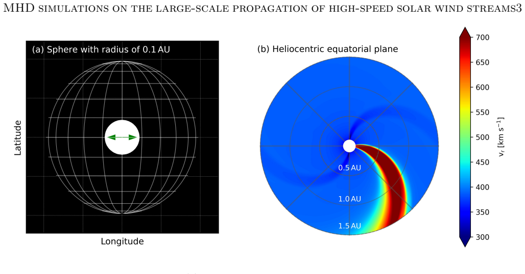
We investigate the propagation of high-speed solar wind streams from their origin near the Sun to 1 AU using three-dimensional magnetohydrodynamic simulations. By tracking both global stream structure and individual plasma parcels, we assess how local in-situ measurements relate to the underlying plasma evolution. We find that high-speed streams are not parcel-preserving structures: commonly used diagnostics such as peak velocity, density, or temperature do not trace fixed plasma elements, and feature-based radial trends can therefore misrepresent the true evolution. Instead, velocity-based relationships provide a more robust framework for linking plasma parcels across heliocentric distances. Stream evolution is dominated by interaction regions, where compression leads to deceleration of fast wind, acceleration of slow wind, and significant heating. A boundary layer forms close to the Sun and can dominate narrow streams, biasing in-situ measurements toward lower apparent velocities. We show that three-dimensional transport, in particular latitudinal flows, redistributes mass and magnetic flux and reduces center-to-flank contrasts. While radial magnetic flux is conserved, the total field strength is not in spherical sampling geometries due to non-radial components. Finally, observed stream properties and geoeffectivity depend strongly on sampling location, stream geometry, and latitudinal magnetic deflection, introducing systematic variability and asymmetries in geomagnetic response.

Editorial analysis

A structured set of objections, weighed in public.

Desk editor's note, referee report, simulated authors' rebuttal, and a circularity audit. Tearing a paper down is the easy half of reading it; the pith above is the substance, this is the friction.

Desk Editor's Note private letter to a colleague

These 3D MHD simulations show high-speed solar wind streams are not parcel-preserving, with latitudinal flows and interaction regions driving the evolution instead of simple radial expansion.

read the letter

The main thing to know is that this paper uses 3D MHD simulations to track both the overall high-speed stream structure and individual plasma parcels as they move out to 1 AU. The central result is that the streams do not preserve plasma parcels: diagnostics like peak velocity or density don't follow the same material, so radial trends based on features can be misleading. Instead, they suggest velocity-based relationships work better for connecting parcels across distances. Stream evolution is dominated by interaction regions that compress and heat the plasma, and a boundary layer forms near the Sun that can skew measurements for narrow streams. Latitudinal flows redistribute mass and flux, cutting down center-to-flank contrasts, while radial magnetic flux stays conserved but total field strength does not in spherical sampling due to non-radial components. Observed properties and geoeffectivity then depend on where you sample and the stream geometry. The work does this with standard ideal MHD and parcel tracking, and the stress-test notes explicit conservation checks with no inconsistencies. That makes the non-preservation finding direct from the dynamics. Soft spots are minor. The work is simulation-based, so it would benefit from more quantitative validation against multi-point observations or sensitivity to parameters like grid resolution, even if the qualitative picture is clear. The abstract doesn't detail those, but assuming the full text has the methods described as standard, it's not a deal-breaker. This paper is for researchers in solar wind propagation and space weather who use or build models linking solar origins to Earth. Readers interested in how 3D effects change simple 1D assumptions will find it relevant. It deserves a serious referee because the claims are grounded in the simulations and have practical implications for data interpretation. I recommend sending it for peer review. The point about non-parcel preservation is worth discussing in the community.

Referee Report

3 major / 3 minor

Summary. The paper presents 3D ideal MHD simulations of high-speed solar wind stream propagation from near the Sun to 1 AU. By advecting passive scalars to track individual plasma parcels alongside the global stream structure, the authors show that streams are not parcel-preserving: peak velocity, density, and temperature at a given radial distance do not correspond to the same plasma elements as they evolve, owing to compression in interaction regions, latitudinal flows, and boundary-layer effects. Velocity-based diagnostics are argued to be more reliable for connecting parcels across distance. Additional results include conservation of radial magnetic flux (but not total |B| in spherical sampling), strong dependence of observed properties on sampling latitude and stream geometry, and the formation of a boundary layer that can bias narrow streams toward lower velocities.

Significance. If the simulations are adequately resolved and validated, the non-preservation result would be a substantive correction to how radial evolution of streams is inferred from in-situ data, with direct consequences for space-weather modeling and the interpretation of stream–stream interaction signatures. The explicit parcel tracking and flux-conservation checks are strengths that allow the central claim to be tested directly from the dynamics rather than assumed.

major comments (3)

[§2 (Numerical Methods)] §2 (Numerical Methods): No grid resolution, cell size, or convergence tests are reported. Because the headline claim rests on the accurate separation of parcel trajectories from feature peaks inside interaction regions, numerical diffusion or under-resolved shear layers could artificially enhance mixing and produce the reported non-preservation; this information is load-bearing.
[§3 (Initial Conditions and Validation)] §3 (Initial Conditions and Validation): The manuscript contains no direct comparison of simulated velocity, density, or magnetic-field profiles at 1 AU against spacecraft observations (e.g., ACE, Wind, or STEREO). Without such validation or at least a quantitative metric of agreement, it is unclear whether the simulated parcel evolution reproduces the observed large-scale structure or is an artifact of the chosen inner-boundary driving.
[§4.3 (Boundary-Layer and Geometry Effects)] §4.3 (Boundary-Layer and Geometry Effects): The claim that a boundary layer “can dominate narrow streams” is presented without a parameter study varying stream width or latitudinal extent. The abstract treats this as a general result, yet the effect’s magnitude and radial onset appear to depend on the specific geometry chosen; a modest sensitivity test would be required to establish how broadly the bias applies.

minor comments (3)

[Abstract] The abstract is lengthy and contains multiple distinct findings; a bulleted summary of the principal results would improve readability.
[Figures] Figure captions for the 3-D renderings should explicitly state the color scale for the passive scalar and the viewing angles used, to allow readers to assess the latitudinal redistribution effect.
[Table 1] A short table summarizing the range of stream widths, speeds, and magnetic-field strengths explored would help readers judge the generality of the reported trends.

Simulated Author's Rebuttal

3 responses · 0 unresolved

We thank the referee for the constructive and detailed report. The comments highlight important aspects of numerical robustness, observational grounding, and generality that will improve the manuscript. We address each major comment below and indicate the revisions we will make.

read point-by-point responses

Referee: §2 (Numerical Methods): No grid resolution, cell size, or convergence tests are reported. Because the headline claim rests on the accurate separation of parcel trajectories from feature peaks inside interaction regions, numerical diffusion or under-resolved shear layers could artificially enhance mixing and produce the reported non-preservation; this information is load-bearing.

Authors: We agree that explicit documentation of resolution and convergence is essential to support the parcel-tracking results. The original submission omitted these details. In the revised manuscript we will expand §2 with the adopted grid (radial, latitudinal, and longitudinal cell counts), the radially varying cell sizes, and the outcomes of resolution-doubling convergence tests. These tests show that the reported non-preservation of parcels, the formation of the boundary layer, and the separation between parcel trajectories and feature peaks remain unchanged at higher resolution, confirming that the effect is dynamical rather than numerical. revision: yes
Referee: §3 (Initial Conditions and Validation): The manuscript contains no direct comparison of simulated velocity, density, or magnetic-field profiles at 1 AU against spacecraft observations (e.g., ACE, Wind, or STEREO). Without such validation or at least a quantitative metric of agreement, it is unclear whether the simulated parcel evolution reproduces the observed large-scale structure or is an artifact of the chosen inner-boundary driving.

Authors: We acknowledge the importance of demonstrating that the simulated large-scale structure is consistent with observations. Our inner-boundary conditions follow standard coronal-hole-driven solar-wind setups used in the literature. In the revision we will add to §3 a direct comparison of the simulated radial velocity, density, and |B| profiles at 1 AU against representative high-speed-stream intervals from ACE and Wind, including quantitative metrics such as peak speed, compression ratio, and magnetic-field magnitude. This will show that the model reproduces the observed bulk properties while the parcel-tracking analysis reveals the underlying dynamical evolution. revision: yes
Referee: §4.3 (Boundary-Layer and Geometry Effects): The claim that a boundary layer “can dominate narrow streams” is presented without a parameter study varying stream width or latitudinal extent. The abstract treats this as a general result, yet the effect’s magnitude and radial onset appear to depend on the specific geometry chosen; a modest sensitivity test would be required to establish how broadly the bias applies.

Authors: The boundary-layer bias is demonstrated for the narrow-stream geometry chosen in the simulation, which is representative of many observed streams. A full parameter sweep over width and latitude would require additional expensive 3D runs. In the revised §4.3 we will (i) qualify the abstract and main text to state that the dominance occurs for narrow streams, (ii) provide a scaling argument based on the existing run and boundary-layer theory, and (iii) note that the effect weakens for wider streams. We believe these clarifications address the generality concern without new simulations. revision: partial

Circularity Check

0 steps flagged

No significant circularity identified

full rationale

The paper derives its central claim—that high-speed streams are not parcel-preserving structures—from independent forward 3D MHD simulations that explicitly track both global stream geometry and individual plasma parcels via passive scalars. The non-preservation result emerges directly from the simulated interaction regions, compression, latitudinal flows, and flux redistribution, without any reduction to fitted parameters, self-definitional relations, or load-bearing self-citations. All reported trends (velocity-based linking, boundary-layer effects, sampling variability) are outputs of the dynamical evolution under standard ideal MHD assumptions, not inputs renamed as predictions. The derivation chain is therefore self-contained against external benchmarks.

Axiom & Free-Parameter Ledger

0 free parameters · 1 axioms · 0 invented entities

The paper's claims depend on the MHD simulation accurately representing real solar wind behavior and the method of tracking individual plasma parcels within the 3D domain.

axioms (1)

domain assumption Ideal MHD equations apply to the solar wind plasma over the scales considered
This is the foundational model used for the simulations.

pith-pipeline@v0.9.0 · 5520 in / 1174 out tokens · 80816 ms · 2026-05-09T17:41:42.225917+00:00 · methodology

discussion (0)

Reference graph

Works this paper leans on

27 extracted references

[1]

C., Ho, G

Allen, R. C., Ho, G. C., Mason, G. M., et al. 2021, Geophys. Res. Lett., 48, e91376

2021
[2]

1977, SoPh, 51, 345

Harvey, J. 1977, SoPh, 51, 345

1977
[3]

Altschuler, M. D. & Newkirk, Jr., G. 1969, SoPh, 9, 131

1969
[4]

Cranmer, S. R. 2002, SSRv, 101, 229 D’Amicis, R., Sorriso-Valvo, L., Benella, S., et al. 2026, A&A, 706, A153

2002
[5]

J., Velli, M

Fox, N. J., Velli, M. C., Bale, S. D., et al. 2016, SSRv, 204, 7

2016
[6]

2022, SoPh, 297, 82

Lockwood, M. 2022, SoPh, 297, 82

2022
[7]

D., Joselyn, J

Gonzalez, W. D., Joselyn, J. A., Kamide, Y., et al. 1994, J. Geophys. Res., 99, 5771

1994
[8]

Gonzalez, W. D. & Tsurutani, B. T. 1987, Planet. Space Sci., 35, 1101 32Hofmeister et al

1987
[9]

Feldman, W. C. 1978, J. Geophys. Res., 83, 1401

1978
[10]

A., Filwett, R

Henderson, S. A., Filwett, R. J., Lee, C. O., et al. 2025, ApJ, 992, 34

2025
[11]

J., Asvestari, E., Guo, J., et al

Hofmeister, S. J., Asvestari, E., Guo, J., et al. 2022, A&A, 659, A190

2022
[12]

C., Klein, K

Kasper, J. C., Klein, K. G., Lichko, E., et al. 2021, PhRvL, 127, 255101

2021
[13]

S., Timothy, A

Krieger, A. S., Timothy, A. F., & Roelof, E. C. 1973, SoPh, 29, 505

1973
[14]

Levine, R. H. 1977, ApJ, 218, 291 M¨ uller, D., St. Cyr, O. C., Zouganelis, I., et al. 2020, A&A, 642, A1 O’Brien, T. P. & McPherron, R. L. 2000, J. Geophys. Res., 105, 7707

1977
[15]

Parker, E. N. 1958, ApJ, 128, 664

1958
[16]

Parker, E. N. 1965, SSRv, 4, 666

1965
[17]

2022, A&A, 668, A189

Perrone, D., Perri, S., Bruno, R., et al. 2022, A&A, 668, A189

2022
[18]

2019, MNRAS, 483, 3730

Matteini, L. 2019, MNRAS, 483, 3730

2019
[19]

& Poedts, S

Pomoell, J. & Poedts, S. 2018, Journal of Space Weather and Space Climate, 8, A35

2018
[20]

Richardson, I. G. 2018, Living Reviews in Solar Physics, 15, 1

2018
[21]

Russell, C. T. & McPherron, R. L. 1973, J. Geophys. Res., 78, 92

1973
[22]

T., Gonzalez, W

Tsurutani, B. T., Gonzalez, W. D., Gonzalez, A. L. C., et al. 2006, Journal of Geophysical Research (Space Physics), 111, A07S01

2006
[23]

Vasyliunas, V. M. 2006, Journal of Geophysical Research (Space Physics), 111, A07S04

2006
[24]

Weber, E. J. & Davis, Jr., L. 1967, ApJ, 148, 217

1967
[25]

Wiegelmann, T., Petrie, G. J. D., & Riley, P. 2017, SSRv, 210, 249

2017
[26]

& Solanki, S

Wiegelmann, T. & Solanki, S. K. 2004, SoPh, 225, 227

2004
[27]

Zirker, J. B. 1977, Reviews of Geophysics and Space Physics, 15, 257

1977