Recognition: unknown
Systematic underestimation of polarisation angle dispersion and its consequences for magnetic field strength estimates in star-forming regions
Pith reviewed 2026-05-07 15:38 UTC · model grok-4.3
The pith
Polarization angle dispersion is systematically underestimated by factors of 1-10 due to pixel size and beam effects, causing magnetic field strengths in star-forming regions to be overestimated.
A machine-rendered reading of the paper's core claim, the machinery that carries it, and where it could break.
Core claim
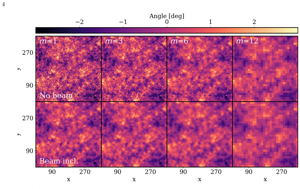
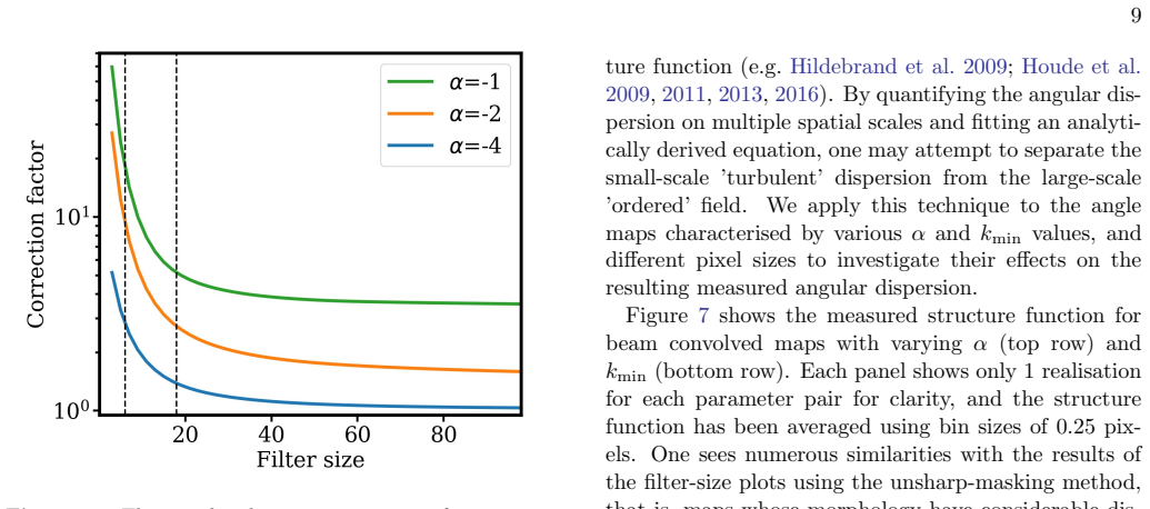
In all cases the measured angular dispersion is underestimated compared to the true value. The degree to which the measured angular dispersion is underestimated varies by factors of 1-10 when measured on scales of 1-3x the beam size, and depends on the underlying structure of the polarisation angle field. This suggests that currently derived magnetic field strengths using angular dispersions are chronically overestimated, potentially leading to an overly magnetically-dominated view of star formation. A method to estimate a correction factor is presented and applied to JCMT Orion A OMC-1 observations, where the field is found to vary on scales much larger than the beam with low unresolveddisp
What carries the argument
Parametrized scale-dependent polarization angle maps analyzed with unsharp-masking and structure-function methods to measure the effect of pixel size and beam convolution on recovered angular dispersion.
Load-bearing premise
The parametrized scale-dependent maps accurately represent the magneto-dynamic turbulence present in real star-forming regions.
What would settle it
Higher-resolution polarization maps of the same region that show the measured dispersion rising by the predicted correction factor as the beam size decreases.
Figures


read the original abstract
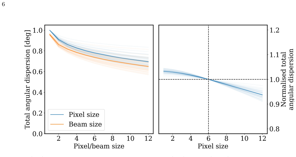
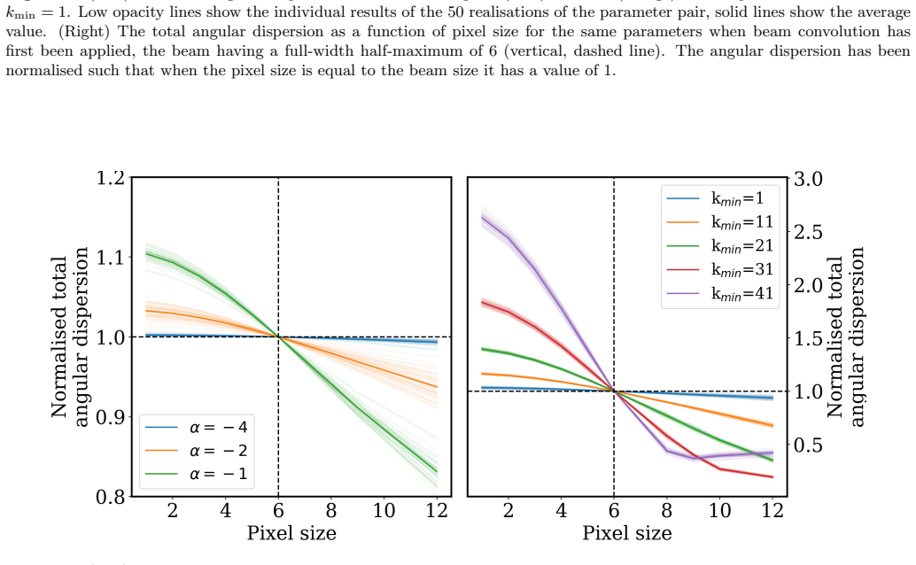
Polarised dust emission observations are a valuable tool to infer the structure of the magnetic field and the dispersion of polarisation position angles may be used to estimate magnetic field strengths. A natural consequence of magneto-dynamic turbulence is for the angular dispersion to have a length-scale dependence, making the measurement of angular dispersion non-trivial. In this paper, we present a study of parametrised, scale dependent maps, focusing on the effect of pixel size and beam convolution on the measured angular dispersion when using the commonly employed unsharp-masking and structure function methods. We find that in all cases the measured angular dispersion is underestimated compared to the true value. The degree to which the measured angular dispersion is underestimated varies by factors of 1-10 when measured on scales of 1-3x the beam size, and depends on the underlying structure of the polarisation angle field. This suggests that currently derived magnetic field strengths using angular dispersions are chronically overestimated, potentially leading to an overly magnetically-dominated view of star formation. We present a method to estimate a correction factor to account for this and apply it to JCMT Orion A OMC-1 observations. We find that the magnetic field in OMC-1 is predominately found to vary on scales much larger than the JCMT's 14'' beam and has a rather low degree of unresolved dispersion, leading to a correction factor of only $\sim$1.6 for angular dispersion measured at a scale of 14''/0.028 pc.
Editorial analysis
A structured set of objections, weighed in public.
Referee Report
Summary. The manuscript examines how finite pixel size and Gaussian beam convolution affect measurements of polarization angle dispersion in scale-dependent fields using unsharp-masking and structure-function estimators. Through a family of parametrized maps, it reports that the measured dispersion is underestimated relative to the true value by factors of 1–10 on scales 1–3 times the beam size. This bias implies that magnetic field strengths derived via the Davis-Chandrasekhar-Fermi method are systematically overestimated. The authors propose a correction procedure based on the parametrized results and apply it to JCMT 850 μm observations of Orion A OMC-1, obtaining a modest correction factor of ∼1.6 that indicates the field varies primarily on scales larger than the 14″ beam with low unresolved dispersion.
Significance. If the reported bias generalizes beyond the chosen parametrizations, the work identifies a previously under-appreciated systematic error in a widely used technique for estimating plane-of-sky magnetic field strengths in star-forming regions. The finding that current B-field estimates may be too high by up to an order of magnitude could alter assessments of magnetic versus turbulent support. The practical correction method and its application to OMC-1 constitute a concrete contribution, though the magnitude of the effect remains tied to the fidelity of the synthetic angle fields.
major comments (3)
- [§3] §3 (construction of parametrized maps): The central results rest on maps generated with explicit functional forms for the scale dependence of the polarization angle field. The manuscript provides no quantitative validation of these forms against either MHD turbulence snapshots or an ensemble of observed polarization maps, nor does it report sensitivity tests to the functional parameters. This leaves open the possibility that the reported underestimation factors (1–10) are specific to the adopted parametrizations rather than generic to magneto-turbulent fields.
- [§4] §4 and abstract (OMC-1 correction): The correction factor of ∼1.6 is obtained by matching the parametrized model to the observed structure function of OMC-1. No formal error propagation, covariance analysis, or Monte-Carlo exploration of model-parameter uncertainty is presented, so the quoted numerical value cannot be assessed for robustness.
- [§2, §5] §2 (methods) and §5 (discussion): The paper does not compare its unsharp-masking and structure-function results on the parametrized maps to the same estimators applied to full MHD simulation cubes with self-consistent density, velocity, and magnetic-field statistics. Such a comparison would directly test whether the bias magnitude or sign changes when the angle field exhibits realistic intermittency and power-spectrum properties.
minor comments (2)
- [Figures] Figure captions (e.g., Fig. 2–4): The exact beam FWHM, pixel scale, and functional parameters used to generate each example map should be stated explicitly in the captions rather than only in the main text.
- [§2] Notation: The distinction between the “true” dispersion (defined on the continuous field) and the “measured” dispersion (after pixelation and convolution) is introduced but not given a compact symbol; introducing a clear notation such as σ_true versus σ_meas would improve readability.
Simulated Author's Rebuttal
We thank the referee for their detailed and constructive report. The comments highlight important aspects of our methodology and the robustness of our conclusions. Below we respond point by point to the major comments, indicating where we agree that revisions are warranted and where we maintain that the current approach is appropriate for the scope of the paper.
read point-by-point responses
-
Referee: §3 (construction of parametrized maps): The central results rest on maps generated with explicit functional forms for the scale dependence of the polarization angle field. The manuscript provides no quantitative validation of these forms against either MHD turbulence snapshots or an ensemble of observed polarization maps, nor does it report sensitivity tests to the functional parameters. This leaves open the possibility that the reported underestimation factors (1–10) are specific to the adopted parametrizations rather than generic to magneto-turbulent fields.
Authors: The parametrized functional forms were selected to isolate the effects of scale dependence, beam convolution, and pixel sampling in a controlled manner, without the additional variables present in full MHD simulations. The chosen forms are motivated by the power-law scale dependence expected in turbulent magnetic fields. We acknowledge that direct quantitative validation against specific MHD snapshots or large observational ensembles was not performed. In the revised manuscript we will add sensitivity tests varying the characteristic scale length and amplitude parameters over ranges consistent with observed polarization maps, demonstrating that the underestimation factors remain between 1 and 10. We will also include a brief discussion relating our parametrizations to typical power spectra reported in the MHD literature. revision: partial
-
Referee: §4 and abstract (OMC-1 correction): The correction factor of ∼1.6 is obtained by matching the parametrized model to the observed structure function of OMC-1. No formal error propagation, covariance analysis, or Monte-Carlo exploration of model-parameter uncertainty is presented, so the quoted numerical value cannot be assessed for robustness.
Authors: We agree that a quantitative assessment of uncertainty in the derived correction factor is desirable. In the revised manuscript we will implement a Monte-Carlo exploration of the parameter space, sampling model parameters that reproduce the observed structure function within its uncertainties. The resulting distribution of correction factors will be reported, allowing readers to evaluate the robustness of the ∼1.6 value for OMC-1. revision: yes
-
Referee: §2 (methods) and §5 (discussion): The paper does not compare its unsharp-masking and structure-function results on the parametrized maps to the same estimators applied to full MHD simulation cubes with self-consistent density, velocity, and magnetic-field statistics. Such a comparison would directly test whether the bias magnitude or sign changes when the angle field exhibits realistic intermittency and power-spectrum properties.
Authors: Our use of parametrized maps was deliberate to separate the influence of scale dependence and observational smoothing from other magneto-hydrodynamic correlations. Introducing full MHD cubes would add density and velocity structure that could obscure the specific bias under study. We recognize the value of such a comparison for establishing generality. In the revised discussion we will expand on how the bias we identify is expected to persist in fields with realistic intermittency, drawing on published MHD polarization statistics, while noting that a direct side-by-side application to MHD cubes lies beyond the present scope. revision: partial
Circularity Check
No circularity: bias quantified directly from constructed maps and applied to independent data
full rationale
The paper constructs its own family of parametrized scale-dependent polarization angle maps, applies the unsharp-masking and structure-function estimators after pixelation and beam convolution, and directly compares the recovered dispersion to the known input dispersion of those same maps. The reported underestimation (factors 1-10 on 1-3 beam scales) is therefore a measured property of the chosen parametrizations, not a reduction of an external claim to a fitted parameter. A correction factor is then derived from the same maps and applied to separate JCMT OMC-1 observations; the observational data are not used to tune the maps or the estimators. No self-citation, uniqueness theorem, or ansatz-smuggling step is present in the provided text, and the derivation chain remains self-contained against the synthetic benchmark it defines.
Axiom & Free-Parameter Ledger
Reference graph
Works this paper leans on
-
[1]
G., Lazarian , A., & Vaillancourt , J
Andersson, B. G., Lazarian, A., & Vaillancourt, J. E. 2015, ARA&A, 53, 501, doi: 10.1146/annurev-astro-082214-122414 Astropy Collaboration, Robitaille, T. P., Tollerud, E. J., et al. 2013, A&A, 558, A33, doi: 10.1051/0004-6361/201322068 Astropy Collaboration, Price-Whelan, A. M., Sip˝ ocz, B. M., et al. 2018, AJ, 156, 123, doi: 10.3847/1538-3881/aabc4f As...
-
[2]
2020, A&A, 636, A39, doi: 10.1051/0004-6361/201936885
Brinkmann, N., Wyrowski, F., Kauffmann, J., et al. 2020, A&A, 636, A39, doi: 10.1051/0004-6361/201936885
-
[3]
1953, ApJ, 118, 113, doi: 10.1086/145731
Chandrasekhar, S., & Fermi, E. 1953, ApJ, 118, 113, doi: 10.1086/145731
-
[4]
Chen, C.-Y., & Ostriker, E. C. 2015, ApJ, 810, 126, doi: 10.1088/0004-637X/810/2/126
-
[5]
2026, Magnetic angular dispersion Correction Factor (MCF) code, Zenodo, doi: 10.5281/zenodo.19202295
Clarke, S. 2026, Magnetic angular dispersion Correction Factor (MCF) code, Zenodo, doi: 10.5281/zenodo.19202295
-
[6]
Cudlip, W., Furniss, I., King, K. J., & Jennings, R. E. 1982, MNRAS, 200, 1169, doi: 10.1093/mnras/200.4.1169
-
[7]
1951, Physical Review, 81, 890, doi: 10.1103/PhysRev.81.890.2
Davis, L. 1951, Physical Review, 81, 890, doi: 10.1103/PhysRev.81.890.2
-
[8]
Davis, L., & Greenstein, J. L. 1949, Physical Review, 75, 1605, doi: 10.1103/PhysRev.75.1605 Falceta-Gon¸ calves, D., Lazarian, A., & Kowal, G. 2008, ApJ, 679, 537, doi: 10.1086/587479 19
-
[9]
2016, Journal of Plasma Physics, 82, 535820601, doi: 10.1017/S0022377816001069
Federrath, C. 2016, Journal of Plasma Physics, 82, 535820601, doi: 10.1017/S0022377816001069
-
[10]
Ganguly, S., Walch, S., Clarke, S. D., & Seifried, D. 2024, MNRAS, 528, 3630, doi: 10.1093/mnras/stae032
-
[11]
Ganguly, S., Walch, S., Seifried, D., Clarke, S. D., & Weis, M. 2023, MNRAS, 525, 721, doi: 10.1093/mnras/stad2054
-
[12]
Gurland, J., & Tripathi, R. C. 1971, The American Statistician, 25, 30, doi: 10.1080/00031305.1971.10477279
-
[13]
Hacar, A., Tafalla, M., & Alves, J. 2017, ArXiv e-prints. https://arxiv.org/abs/1703.07029
-
[14]
Harris, C. R., Millman, K. J., van der Walt, S. J., et al. 2020, Nature, 585, 357, doi: 10.1038/s41586-020-2649-2
-
[15]
Norman, M. L. 2001, ApJ, 561, 800, doi: 10.1086/323489
-
[16]
Hildebrand, R. H. 1988, QJRAS, 29, 327
1988
-
[17]
Hildebrand, R. H., Dragovan, M., & Novak, G. 1984, ApJL, 284, L51, doi: 10.1086/184351
-
[18]
Vaillancourt, J. E. 2009, ApJ, 696, 567, doi: 10.1088/0004-637X/696/1/567
-
[19]
Hiltner, W. A. 1949, Science, 109, 165, doi: 10.1126/science.109.2825.165
-
[20]
Hoang, T., Tram, L. N., Lee, H., Diep, P. N., & Ngoc, N. B. 2021, ApJ, 908, 218, doi: 10.3847/1538-4357/abd54f
-
[21]
2013, ApJ, 766, 49, doi: 10.1088/0004-637X/766/1/49
Houde, M., Fletcher, A., Beck, R., et al. 2013, ApJ, 766, 49, doi: 10.1088/0004-637X/766/1/49
-
[22]
Houde, M., Hull, C. L. H., Plambeck, R. L., Vaillancourt, J. E., & Hildebrand, R. H. 2016, ApJ, 820, 38, doi: 10.3847/0004-637X/820/1/38
-
[23]
Houde, M., Rao, R., Vaillancourt, J. E., & Hildebrand, R. H. 2011, ApJ, 733, 109, doi: 10.1088/0004-637X/733/2/109
-
[24]
Chitsazzadeh, S., & Kirby, L. 2009, ApJ, 706, 1504, doi: 10.1088/0004-637X/706/2/1504
-
[25]
Hull, C. L. H., Plambeck, R. L., Kwon, W., et al. 2014, ApJS, 213, 13, doi: 10.1088/0067-0049/213/1/13
-
[26]
Hull, C. L. H., Mocz, P., Burkhart, B., et al. 2017, ApJL, 842, L9, doi: 10.3847/2041-8213/aa71b7
-
[27]
Hunter, J. D. 2007, Computing in Science and Engineering, 9, 90, doi: 10.1109/MCSE.2007.55
-
[28]
2021, , 913, 85, 10.3847/1538-4357/abf3c4
Hwang, J., Kim, J., Pattle, K., et al. 2021, ApJ, 913, 85, doi: 10.3847/1538-4357/abf3c4 Ib´ a˜ nez-Mej´ ıa, J. C., Mac Low, M.-M., & Klessen, R. S. 2022, ApJ, 925, 196, doi: 10.3847/1538-4357/ac3b58
-
[29]
2018, , 70, S53, 10.1093/pasj/psx089
Inoue, T., Hennebelle, P., Fukui, Y., et al. 2018, PASJ, 70, S53, doi: 10.1093/pasj/psx089
-
[30]
2012, A&A, 543, A128, doi: 10.1051/0004-6361/201118730
Joos, M., Hennebelle, P., & Ciardi, A. 2012, A&A, 543, A128, doi: 10.1051/0004-6361/201118730
-
[31]
Kim, J.-G., Ostriker, E. C., & Filippova, N. 2021, ApJ, 911, 128, doi: 10.3847/1538-4357/abe934
-
[32]
Koch, P. M., Tang, Y.-W., Ho, P. T. P., et al. 2014, ApJ, 797, 99, doi: 10.1088/0004-637X/797/2/99
-
[33]
2018, , 859, 4, 10.3847/1538-4357/aabd82
Kwon, J., Doi, Y., Tamura, M., et al. 2018, ApJ, 859, 4, doi: 10.3847/1538-4357/aabd82
-
[34]
2007, MNRAS, 378, 910, doi: 10.1111/j.1365-2966.2007.11817.x
Lazarian, A., & Hoang, T. 2007, MNRAS, 378, 910, doi: 10.1111/j.1365-2966.2007.11817.x
-
[35]
Lazarian, A., Yuen, K. H., & Pogosyan, D. 2022, ApJ, 935, 77, doi: 10.3847/1538-4357/ac6877
-
[36]
2021, ApJ, 918, 39, doi: 10.3847/1538-4357/ac0cf2
Lee, D., Berthoud, M., Chen, C.-Y., et al. 2021, ApJ, 918, 39, doi: 10.3847/1538-4357/ac0cf2
-
[37]
S., Lopez-Rodriguez, E., Ajeddig, H., et al
Li, P. S., Lopez-Rodriguez, E., Ajeddig, H., et al. 2022, MNRAS, 510, 6085, doi: 10.1093/mnras/stab3448
-
[38]
2021, ApJ, 919, 79, doi: 10.3847/1538-4357/ac0cec
Liu, J., Zhang, Q., Commer¸ con, B., et al. 2021, ApJ, 919, 79, doi: 10.3847/1538-4357/ac0cec
-
[39]
2022, Frontiers in Astronomy and Space Sciences, 9, 943556, doi: 10.3389/fspas.2022.943556
Liu, J., Zhang, Q., & Qiu, K. 2022, Frontiers in Astronomy and Space Sciences, 9, 943556, doi: 10.3389/fspas.2022.943556
-
[40]
Lomax, O., Whitworth, A. P., & Hubber, D. A. 2015, MNRAS, 449, 662, doi: 10.1093/mnras/stv310
-
[41]
Menten, K. M., Reid, M. J., Forbrich, J., & Brunthaler, A. 2007, A&A, 474, 515, doi: 10.1051/0004-6361:20078247
-
[42]
1956, MNRAS, 116, 503, 10.1093/MNRAS/116.5.503
Mestel, L., & Spitzer, L., J. 1956, MNRAS, 116, 503, doi: 10.1093/mnras/116.5.503
-
[43]
Myers, P. C., & Goodman, A. A. 1991, ApJ, 373, 509, doi: 10.1086/170070
-
[44]
Ngoc, N. B., Diep, P. N., Hoang, T., et al. 2023, ApJ, 953, 66, doi: 10.3847/1538-4357/acdb6e
-
[45]
Ostriker, E. C., Stone, J. M., & Gammie, C. F. 2001, ApJ, 546, 980, doi: 10.1086/318290
-
[46]
Padoan, P., Goodman, A., Draine, B. T., et al. 2001, ApJ, 559, 1005, doi: 10.1086/322504
-
[47]
2019, Frontiers in Astronomy and Space Sciences, 6, 15, doi: 10.3389/fspas.2019.00015
Pattle, K., & Fissel, L. 2019, Frontiers in Astronomy and Space Sciences, 6, 15, doi: 10.3389/fspas.2019.00015
-
[48]
2023, in Astronomical Society of the Pacific Conference
Pattle, K., Fissel, L., Tahani, M., Liu, T., & Ntormousi, E. 2023, in Astronomical Society of the Pacific Conference
2023
-
[49]
2017, , 846, 122, 10.3847/1538-4357/aa80e5
Pattle, K., Ward-Thompson, D., Berry, D., et al. 2017, ApJ, 846, 122, doi: 10.3847/1538-4357/aa80e5
-
[50]
Pillai, T. G. S., Clemens, D. P., Reissl, S., et al. 2020, Nature Astronomy, 4, 1195, doi: 10.1038/s41550-020-1172-6
-
[51]
2020, , 641, A12, 10.1051/0004-6361/201833885
Pineda, J. E., Arzoumanian, D., Andre, P., et al. 2023, in Astronomical Society of the Pacific Conference Series, Vol. 534, Astronomical Society of the Pacific Conference Series, ed. S. Inutsuka, Y. Aikawa, T. Muto, K. Tomida, & M. Tamura, 233 20 Planck Collaboration, Aghanim, N., Akrami, Y., et al. 2020, A&A, 641, A12, doi: 10.1051/0004-6361/201833885
-
[52]
Schive, H.-Y., ZuHone, J. A., Goldbaum, N. J., et al. 2018, MNRAS, 481, 4815, doi: 10.1093/mnras/sty2586
-
[53]
Pudritz, R. E. 2011, MNRAS, 417, 1054, doi: 10.1111/j.1365-2966.2011.19320.x
-
[54]
Bisbas, T. G. 2020, MNRAS, 492, 1465, doi: 10.1093/mnras/stz3563
-
[55]
2021, A&A, 656, A118, doi: 10.1051/0004-6361/202142045
Tassis, K. 2021, A&A, 656, A118, doi: 10.1051/0004-6361/202142045
-
[56]
Tang, Y.-W., Koch, P. M., Peretto, N., et al. 2019, ApJ, 878, 10, doi: 10.3847/1538-4357/ab1484
-
[57]
Virtanen, P., Gommers, R., Oliphant, T. E., et al. 2020, Nature Methods, 17, 261, doi: 10.1038/s41592-019-0686-2
-
[58]
2019, , 876, 42, 10.3847/1538-4357/ab13a2
Wang, J.-W., Lai, S.-P., Eswaraiah, C., et al. 2019, ApJ, 876, 42, doi: 10.3847/1538-4357/ab13a2
-
[59]
Wang, J.-W., Koch, P. M., Clarke, S. D., et al. 2024, ApJ, 962, 136, doi: 10.3847/1538-4357/ad165b
-
[60]
2017, , 842, 66, 10.3847/1538-4357/aa70a0
Ward-Thompson, D., Pattle, K., Bastien, P., et al. 2017, ApJ, 842, 66, doi: 10.3847/1538-4357/aa70a0
-
[61]
Whittet, D. C. B., Hough, J. H., Lazarian, A., & Hoang, T. 2008, ApJ, 674, 304, doi: 10.1086/525040
-
[62]
Wiebe, D. S., & Watson, W. D. 2004, ApJ, 615, 300, doi: 10.1086/424033
-
[63]
doi:10.1093/mnras/stz2215 , eprint =
Wurster, J., Bate, M. R., & Price, D. J. 2019, MNRAS, 489, 1719, doi: 10.1093/mnras/stz2215
-
[64]
Wurster, J., Price, D. J., & Bate, M. R. 2016, MNRAS, 457, 1037, doi: 10.1093/mnras/stw013
discussion (0)
Sign in with ORCID, Apple, or X to comment. Anyone can read and Pith papers without signing in.