arxiv: 2605.03881 · v1 · submitted 2026-05-05 · 💰 econ.GN · q-fin.EC

Recognition: unknown

Fiscal Aggregation and the Limits of IS--LM--BP: Derivations, Aggregation Bias and Reproducible Adversarial Simulations

Ricardo Alonzo Fernandez Salguero

Pith reviewed 2026-05-07 12:30 UTC · model grok-4.3

classification 💰 econ.GN q-fin.EC

keywords fiscal aggregationIS-LM-BPaggregation biasfiscal multipliersopen economyfiscal compositionMundell-Flemingpublic investment

0 comments

The pith

The aggregate fiscal variable G suffices for output analysis only if every instrument has the identical marginal effect on output.

A machine-rendered reading of the paper's core claim, the machinery that carries it, and where it could break.

The paper establishes that scalar aggregation of fiscal policy into a single G variable in the IS-LM-BP framework holds only when all components—current purchases, public investment, and transfers—share the same marginal impact on output. It derives the precise gradient condition that makes this true, shows how violations produce aggregation bias, and constructs composition-weighted multipliers. The work then extends the open-economy model to track fiscal composition, public capital, debt dynamics, and risk premia while confirming internal consistency through symbolic derivations and adversarial simulations. A sympathetic reader cares because standard multiplier estimates and policy rules rest on the assumption that total spending alone determines outcomes.

Core claim

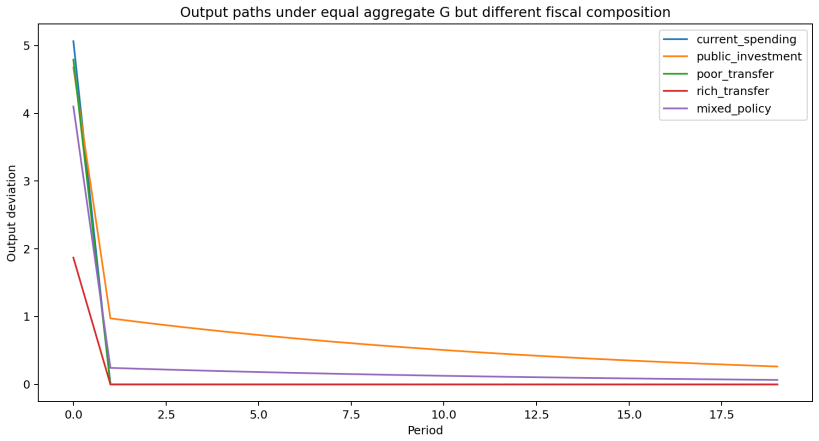
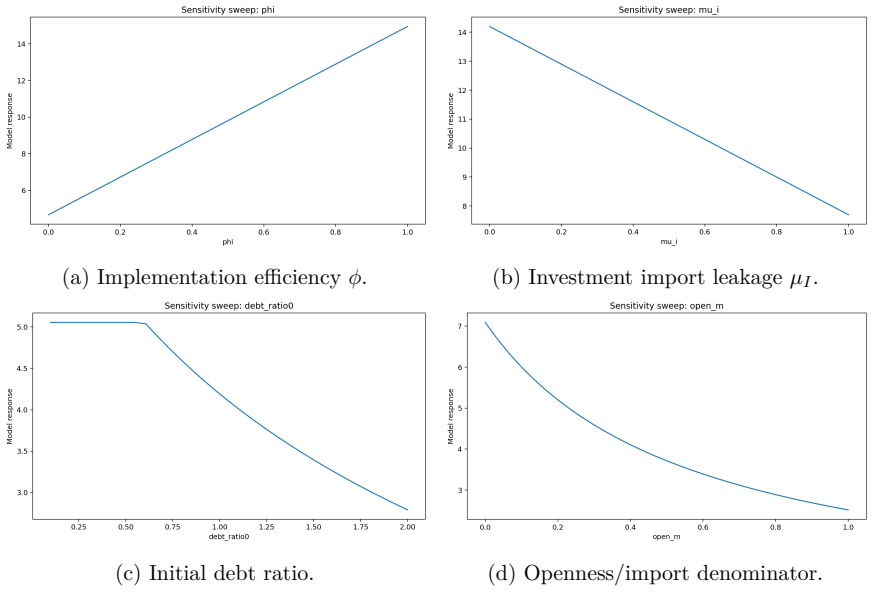
When fiscal policy consists of heterogeneous instruments, the scalar aggregate G is sufficient for output analysis only under the restrictive gradient condition that all instruments exert identical marginal effects on output; otherwise, composition-weighted multipliers must replace the single variable, and the IS-LM-BP model must incorporate fiscal composition, public capital, debt dynamics, and risk-premium effects. The paper proves the condition, identifies the resulting aggregation bias, and verifies the extended framework through reproducible symbolic checks, derivative tests, accounting identities, adversarial counterexamples, sensitivity sweeps, Monte Carlo simulations, and stress test

What carries the argument

the gradient condition requiring identical marginal output effects across all fiscal instruments, which determines when scalar aggregation is valid and when vector-valued, state-contingent multipliers are required instead

If this is right

Fiscal policy analysis must treat instruments as a vector rather than a scalar sum.
Multipliers become state-contingent and depend on the specific mix of purchases, investment, and transfers.
Standard IS-LM-BP forecasts that ignore composition will contain systematic bias.
Policy rules and empirical estimates require explicit tracking of fiscal composition and debt feedback.
The extended model preserves the compact equilibrium representation while adding the necessary detail.

Where Pith is reading between the lines

These are editorial extensions of the paper, not claims the author makes directly.

Empirical studies that rely on aggregate spending data may systematically mis-estimate multipliers whenever the instrument mix changes across episodes.
Optimal stimulus design should target the composition of spending rather than its total size to achieve a given output goal at lower cost.
The same aggregation logic could be applied to other macro models that currently collapse government spending into a single variable.
Reproducible adversarial testing of this kind could be used to audit other compact representations in open-economy macroeconomics.

Load-bearing premise

That the marginal effects of heterogeneous fiscal instruments can be separately identified within an extended IS-LM-BP equilibrium that still remains useful once composition, public capital, debt, and risk-premium terms are added.

What would settle it

A simulation or empirical case in which fiscal instruments with measurably different marginal effects on output nevertheless produce the same aggregate output response as predicted by scalar G alone, with no detectable composition bias.

Figures

Figures reproduced from arXiv: 2605.03881 by Ricardo Alonzo Fernandez Salguero.

**Figure 1.** Figure 1: Output paths under equal aggregate spending but different fiscal composition. view at source ↗

**Figure 2.** Figure 2: Monte Carlo distribution of present-value output by fiscal composition. view at source ↗

**Figure 3.** Figure 3: Sensitivity sweeps. the accounting equations hold, whether counterexamples behave as expected, and whether the scalar-G model fails under heterogeneous instruments. 23 view at source ↗

read the original abstract

This paper develops a formal critique of scalar fiscal aggregation in the IS LM BP/Mundell Fleming framework. It shows that when fiscal policy is composed of heterogeneous instruments current purchases, public investment and transfers to different households the aggregate variable G is sufficient for output analysis only under a restrictive gradient condition: all instruments must have identical marginal effects on output. The paper proves this condition, derives composition weighted multipliers, identifies aggregation bias and extends the open economy IS LM BP model to incorporate fiscal composition, public capital, debt dynamics and risk-premium effects. A reproducible computational exercise with symbolic checks, derivative tests, accounting identities, adversarial counterexamples, sensitivity sweeps, Monte Carlo simulations and stress tests confirms the internal consistency of the argument. The contribution is methodological: IS LM BP remains useful as a compact equilibrium framework, but fiscal policy analysis requires vector-valued instruments and state-contingent multipliers rather than a single homogeneous spending variable.

Editorial analysis

A structured set of objections, weighed in public.

Desk editor's note, referee report, simulated authors' rebuttal, and a circularity audit. Tearing a paper down is the easy half of reading it; the pith above is the substance, this is the friction.

Desk Editor's Note private letter to a colleague

Scalar G in IS-LM-BP works only if fiscal instruments share identical marginal output effects, and the paper derives the condition with weighted multipliers plus reproducible simulations to show the bias.

read the letter

The main point is that the aggregate fiscal variable G is reliable in the open-economy IS-LM-BP model only when all instruments have the same marginal effect on output. The paper derives this gradient condition, works out the composition-weighted multipliers, and extends the framework to cover public capital, debt dynamics, and risk premia while keeping the equilibrium solution method intact. Adversarial simulations and Monte Carlo runs then illustrate the aggregation bias when the condition fails. This is useful formal work within the model and the computational checks are transparent and reproducible. The derivations appear self-contained and the stress tests align with the algebra without obvious circularity. The soft spots are that the base IS-LM-BP setup is already quite stylized, so adding layers of fiscal detail preserves the compact form but does not overcome its broader limitations in dynamics or expectations. The gradient condition itself follows directly from requiring the total derivative to be independent of composition, so the advance is more in the explicit treatment and verification than in a deep surprise. The paper assumes separate marginal effects can be identified for the theory, which is reasonable for the exercise but would need care in applications. This is mainly for researchers or instructors who still use or teach the Mundell-Fleming framework and want to handle fiscal composition more precisely. It shows clear engagement with the math and verification steps, so it deserves peer review rather than a desk reject.

Referee Report

0 major / 3 minor

Summary. The paper claims that scalar fiscal aggregation into a single G variable in the IS-LM-BP (Mundell-Fleming) framework is valid for output determination only under a restrictive gradient condition requiring identical marginal effects across heterogeneous instruments (current purchases, public investment, transfers). It proves this condition, derives composition-weighted multipliers, identifies resulting aggregation bias, extends the model to incorporate public capital accumulation, debt dynamics, and endogenous risk premia while preserving equilibrium solution methods, and verifies internal consistency via symbolic checks, derivative tests, accounting identities, adversarial counterexamples, sensitivity sweeps, Monte Carlo simulations, and stress tests.

Significance. If the derivations and simulations hold, the work offers a clear methodological contribution by showing that IS-LM-BP remains a compact equilibrium framework but requires vector-valued fiscal instruments and state-contingent multipliers rather than homogeneous G. The reproducible adversarial simulations and Monte Carlo exercises, including explicit tests of gradient-condition violations, provide falsifiable verification that strengthens the central claim about aggregation bias.

minor comments (3)

[Abstract and computational exercise] The abstract and simulation sections reference 'symbolic checks' and 'reproducible computational exercise' but do not name the specific software, libraries, or code repository used, which would aid full reproducibility.
[Simulation and stress-test sections] Monte Carlo and adversarial simulation descriptions would benefit from explicit reporting of random seeds, exact parameter draws, and the precise functional forms used for heterogeneous marginal effects to allow direct replication of the bias results.
[Model extension] Notation for the total derivative dY/dG and the gradient condition could be stated more explicitly when the model is extended with public capital and risk premia to avoid ambiguity in how composition weights enter the equilibrium.

Simulated Author's Rebuttal

0 responses · 0 unresolved

We thank the referee for the positive and accurate summary of our manuscript, as well as for the recommendation of minor revision. The referee's assessment correctly captures our central methodological contribution on the restrictive conditions for scalar fiscal aggregation in the IS-LM-BP framework and the value of the reproducible verification exercises.

Circularity Check

0 steps flagged

Derivation self-contained; no circular steps

full rationale

The core claim—that scalar G suffices for output only when all fiscal instruments share identical marginal effects—is derived directly from the total derivative dY/dG being independent of composition in the extended IS-LM-BP equations. This follows from the model's accounting identities and equilibrium conditions without redefinition or fitting. Extensions for public capital, debt dynamics, and risk premia are added while preserving the solution method; adversarial Monte Carlo tests and symbolic checks confirm internal consistency but do not serve as load-bearing inputs. No self-citations are invoked for uniqueness theorems or ansatzes, and no parameter is fitted then relabeled as a prediction. The chain is mathematically independent of its own outputs.

Axiom & Free-Parameter Ledger

0 free parameters · 0 axioms · 0 invented entities

Only the abstract is available; no explicit free parameters, axioms, or invented entities can be extracted or verified. The paper refers to standard macroeconomic accounting identities and derivative conditions but supplies no further detail.

pith-pipeline@v0.9.0 · 5463 in / 1275 out tokens · 77313 ms · 2026-05-07T12:30:34.742944+00:00 · methodology

discussion (0)

Reference graph

Works this paper leans on

32 extracted references · 28 canonical work pages

[1]

Abiad, A., Furceri, D., and Topalova, P. (2016). The macroeconomic effects of public investment: Evidence from advanced economies.Journal of Macroeconomics, 50, 224– 240.https://doi.org/10.1016/j.jmacro.2016.07.005

work page doi:10.1016/j.jmacro.2016.07.005 2016
[2]

Auclert, A., Bardóczy, B., Rognlie, M., and Straub, L. (2021). Using the sequence- space Jacobian to solve and estimate heterogeneous-agent models.Econometrica, 89(5), 2375–2408.https://doi.org/10.3982/ECTA17434

work page doi:10.3982/ecta17434 2021
[3]

Auerbach, A. J. and Gorodnichenko, Y. (2012). Measuring the output responses to fiscal policy.American Economic Journal: Economic Policy, 4(2), 1–27.https://doi.org/ 10.1257/pol.4.2.1

work page doi:10.1257/pol.4.2.1 2012
[4]

Blanchard, O. J. and Leigh, D. (2013). Growth forecast errors and fiscal multipliers. American Economic Review, 103(3), 117–120.https://doi.org/10.1257/aer.103.3. 117

work page doi:10.1257/aer.103.3 2013
[5]

and Perotti, R

Blanchard, O. and Perotti, R. (2002). An empirical characterization of the dynamic effects of changes in government spending and taxes on output.The Quarterly Journal of Economics, 117(4), 1329–1368.https://doi.org/10.1162/003355302320935043 30

work page doi:10.1162/003355302320935043 2002
[6]

Bohn, H. (1998). The behavior of U.S. public debt and deficits.The Quarterly Journal of Economics, 113(3), 949–963.https://doi.org/10.1162/003355398555793

work page doi:10.1162/003355398555793 1998
[7]

Bom, P. R. D. and Ligthart, J. E. (2014). What have we learned from three decades of research on the productivity of public capital?Journal of Economic Surveys, 28(5), 889–916.https://doi.org/10.1111/joes.12037

work page doi:10.1111/joes.12037 2014
[8]

Calvo, G. A. (1998). Capital flows and capital-market crises: The simple economics of sudden stops.Journal of Applied Economics, 1(1), 35–54.https://doi.org/10.1080/ 15140326.1998.12040516

work page arXiv 1998
[9]

Clarida, R., Galí, J., and Gertler, M. (1999). The science of monetary policy: A New Keynesian perspective.Journal of Economic Literature, 37(4), 1661–1707.https: //doi.org/10.1257/jel.37.4.1661

work page doi:10.1257/jel.37.4.1661 1999
[10]

Dornbusch, R. (1976). Expectations and exchange rate dynamics.Journal of Political Economy, 84(6), 1161–1176.https://doi.org/10.1086/260506

work page doi:10.1086/260506 1976
[11]

Fleming, J. M. (1962). Domestic financial policies under fixed and under floating exchange rates.IMF Staff Papers, 9(3), 369–380.https://doi.org/10.2307/3866091

work page doi:10.2307/3866091 1962
[12]

Gechert, S. (2015). What fiscal policy is most effective? A meta-regression analysis.Oxford Economic Papers, 67(3), 553–580.https://doi.org/10.1093/oep/gpv027

work page doi:10.1093/oep/gpv027 2015
[13]

and Rannenberg, A

Gechert, S. and Rannenberg, A. (2018). Which fiscal multipliers are regime-dependent? A meta-regression analysis.Journal of Economic Surveys, 32(4), 1160–1182.https: //doi.org/10.1111/joes.12241

work page doi:10.1111/joes.12241 2018
[14]

Mr. Keynes and the "Classics"; A Suggested Interpretation

Hicks, J. R. (1937). Mr. Keynes and the “Classics”: A suggested interpretation.Econo- metrica, 5(2), 147–159.https://doi.org/10.2307/1907242

work page doi:10.2307/1907242 1937
[15]

A., Lim, J

Huidrom, R., Kose, M. A., Lim, J. J., and Ohnsorge, F. L. (2020). Why do fiscal multipliers depend on fiscal positions?Journal of Monetary Economics, 114, 109–125. https://doi.org/10.1016/j.jmoneco.2019.03.004

work page doi:10.1016/j.jmoneco.2019.03.004 2020
[16]

G., and Végh, C

Ilzetzki, E., Mendoza, E. G., and Végh, C. A. (2013). How big (small?) are fiscal multipliers?Journal of Monetary Economics, 60(2), 239–254.https://doi.org/10.1 016/j.jmoneco.2012.10.011

2013
[17]

M., and Rogoff, K

Ilzetzki, E., Reinhart, C. M., and Rogoff, K. S. (2019). Exchange arrangements entering the twenty-first century: Which anchor will hold?The Quarterly Journal of Economics, 134(2), 599–646.https://doi.org/10.1093/qje/qjy033 31 International Monetary Fund. (2014). Is it time for an infrastructure push? The macroeco- nomic effects of public investment. InWo...

work page doi:10.1093/qje/qjy033 2019
[18]

Clouds, Uncertainties, Chapter 3.https://www.imf.org/-/media/Websites/IMF/i mported-flagship-issues/external/pubs/ft/weo/2014/02/pdf/_c3pdf.pdf

2014
[19]

and Violante, G

Kaplan, G. and Violante, G. L. (2014). A model of the consumption response to fiscal stimulus payments.Econometrica, 82(4), 1199–1239.https://doi.org/10.3982/ECTA 10528

work page doi:10.3982/ecta 2014
[20]

Kaplan, G., Moll, B., and Violante, G. L. (2018). Monetary policy according to HANK. American Economic Review, 108(3), 697–743.https://doi.org/10.1257/aer.2016 0042

work page doi:10.1257/aer.2016 2018
[21]

Kraay, A. (2012). How large is the government spending multiplier? Evidence from World Bank lending.The Quarterly Journal of Economics, 127(2), 829–887.https: //doi.org/10.1093/qje/qjs008

work page doi:10.1093/qje/qjs008 2012
[22]

Kraay, A. (2014). Government spending multipliers in developing countries.American Economic Journal: Macroeconomics, 6(4), 170–208.https://doi.org/10.1257/mac. 6.4.170

work page doi:10.1257/mac 2014
[23]

M., Walker, T

Leeper, E. M., Walker, T. B., and Yang, S.-C. S. (2010). Government investment and fiscal stimulus.Journal of Monetary Economics, 57(8), 1000–1012.https://doi.org/ 10.1016/j.jmoneco.2010.09.002

work page doi:10.1016/j.jmoneco.2010.09.002 2010
[24]

and Uhlig, H

Mountford, A. and Uhlig, H. (2009). What are the effects of fiscal policy shocks?Journal of Applied Econometrics, 24(6), 960–992.https://doi.org/10.1002/jae.1079

work page doi:10.1002/jae.1079 2009
[25]

Mundell, R. A. (1963). Capital mobility and stabilization policy under fixed and flexible exchange rates.Canadian Journal of Economics and Political Science, 29(4), 475–485. https://doi.org/10.2307/139336

work page doi:10.2307/139336 1963
[26]

and Steinsson, J

Nakamura, E. and Steinsson, J. (2014). Fiscal stimulus in a monetary union: Evidence from US regions.American Economic Review, 104(3), 753–792.https://doi.org/10 .1257/aer.104.3.753

2014
[27]

A., Souleles, N

Parker, J. A., Souleles, N. S., Johnson, D. S., and McClelland, R. (2013). Consumer spending and the economic stimulus payments of 2008.American Economic Review, 103(6), 2530–2553.https://doi.org/10.1257/aer.103.6.2530

work page doi:10.1257/aer.103.6.2530 2013
[28]

Perotti, R. (2005). Estimating the effects of fiscal policy in OECD countries. CEPR Discussion Paper No. 4842.https://cepr.org/publications/dp4842 32

2005
[29]

Ramey, V. A. (2019). Ten years after the financial crisis: What have we learned from the renaissance in fiscal research?Journal of Economic Perspectives, 33(2), 89–114. https://doi.org/10.1257/jep.33.2.89

work page doi:10.1257/jep.33.2.89 2019
[30]

Ramey, V. A. and Zubairy, S. (2018). Government spending multipliers in good times and in bad: Evidence from U.S. historical data.Journal of Political Economy, 126(2), 850–901.https://doi.org/10.1086/696277

work page doi:10.1086/696277 2018
[31]

Reinhart, C. M. and Rogoff, K. S. (2004). The modern history of exchange rate ar- rangements: A reinterpretation.The Quarterly Journal of Economics, 119(1), 1–48. https://doi.org/10.1162/003355304772839515

work page doi:10.1162/003355304772839515 2004
[32]

Romer, D. H. (2000). Keynesian macroeconomics without the LM curve.Journal of Economic Perspectives, 14(2), 149–169.https://doi.org/10.1257/jep.14.2.149 33

work page doi:10.1257/jep.14.2.149 2000