Recognition: unknown
Raising the Ceiling: Better Empirical Fixation Densities for Saliency Benchmarking
Pith reviewed 2026-05-07 17:26 UTC · model grok-4.3
The pith
A per-image mixture model for fixation densities raises measured interobserver consistency by 5-15% over standard Gaussian kernels.
A machine-rendered reading of the paper's core claim, the machinery that carries it, and where it could break.
Core claim
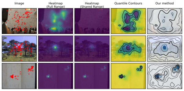
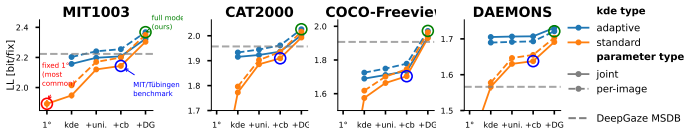
By modeling fixation locations as a mixture of an adaptive-bandwidth KDE based on Abramson's method, center bias and uniform components, and a state-of-the-art saliency model, with all parameters optimized per image via leave-one-subject-out cross-validation, the resulting densities achieve substantially higher agreement with held-out observers than fixed-bandwidth isotropic Gaussian KDE, yielding median per-image gains of 5-15% in log-likelihood and up to 2 percentage points in AUC, with improvements exceeding 25% on the most affected images.
What carries the argument
A per-image mixture model that combines Abramson's adaptive-bandwidth kernel density estimate, center bias, uniform distribution, and a state-of-the-art saliency model, with mixture weights and bandwidths optimized via leave-one-subject-out cross-validation to capture different types of interobserver consistency.
If this is right
- Median per-image gains of 5-15% in log-likelihood and up to 2 percentage points in AUC when predicting held-out fixations.
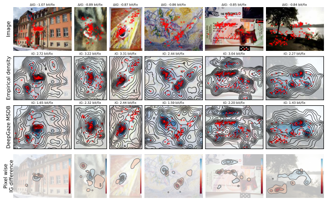
- Improvements exceed 25% precisely on the images most relevant to failure case analysis.
- The new densities allow identification of remaining failure cases of state-of-the-art saliency models, indicating significant headroom for further model improvement.
- Empirical fixation densities should be treated as evolving estimates that improve with better methodology rather than fixed ground truths.
Where Pith is reading between the lines
- Switching to these densities would likely re-rank which images count as current model failures and could shift priorities in future failure-case studies.
- The same adaptive mixture approach could be applied to other point-pattern data, such as mouse clicks or trajectory traces, to obtain more reliable density estimates.
- A controlled experiment that applies the method to new eye-tracking datasets without including any saliency model in the mixture would test how much of the reported gain depends on that component.
- If widely adopted, benchmark conclusions about the sufficiency of existing saliency models would need to be revisited with the updated consistency ceiling.
Load-bearing premise
Including a state-of-the-art saliency model as one mixture component together with per-image parameter optimization via leave-one-subject-out cross-validation produces an unbiased estimate of human interobserver consistency rather than partially fitting the model to the benchmark data.
What would settle it
A side-by-side saliency benchmark comparison that shows whether the set of remaining model failure cases or the relative model rankings change when the new densities replace the standard Gaussian KDE densities, or a test that removes the saliency model component and checks whether the consistency gains largely disappear.
Figures


read the original abstract
Empirical fixation densities, spatial distributions estimated from human eye-tracking data, are foundational to saliency benchmarking. They directly shape benchmark conclusions, leaderboard rankings, failure case analyses, and scientific claims about human visual behavior. Yet the standard estimation method, fixed-bandwidth isotropic Gaussian KDE, has gone essentially unchanged for decades. This matters now more than ever: as the field shifts toward sample-level evaluation (failure case analysis, inverse benchmarking, per-image model comparison), reliable per-image density estimates become critical. We propose a principled mixture model that combines an adaptive-bandwidth KDE based on Abramson's method, center bias and uniform components, and a state-of-the-art saliency model, to capture different spatial and semantic types of interobserver consistency, and optimize all parameters per image via leave-one-subject-out cross-validation. Our method yields substantially higher interobserver consistency estimates across multiple benchmarks, with median per-image gains of 5-15% in log-likelihood and up to 2 percentage points in AUC. For the most affected images -- precisely those most relevant to failure case analysis -- improvements exceed 25%. We leverage these improved estimates to identify and analyze remaining failure cases of state-of-the-art saliency models, demonstrating that significant headroom for model improvement remains. More broadly, our findings highlight that empirical fixation densities should not be treated as fixed ground truths but as evolving estimates that improve with better methodology.
Editorial analysis
A structured set of objections, weighed in public.
Referee Report
Summary. The manuscript claims that standard fixed-bandwidth isotropic Gaussian KDE for empirical fixation densities is insufficient for modern saliency benchmarking, especially sample-level analysis. It proposes a four-component mixture (Abramson adaptive KDE + center bias + uniform + one external SOTA saliency model) whose weights and bandwidths are fit per image via LOOCV. This yields median per-image gains of 5-15% log-likelihood and up to 2 pp AUC in inter-observer consistency, with >25% gains on failure-case images, which the authors then use to argue that substantial headroom remains for SOTA saliency models.
Significance. If the estimator is unbiased, the work would be significant for the field: it would show that conventional densities systematically underestimate human consistency, revise failure-case analyses, and tighten the evaluation of model progress. The per-image optimization and explicit mixture of spatial/semantic components are methodologically interesting strengths. Credit is given for the focus on per-image metrics and the attempt to move beyond fixed KDE.
major comments (2)
- [Abstract and §3] Abstract and §3 (mixture construction): the estimator includes a SOTA saliency model as an explicit component whose weight is chosen by per-image LOOCV on the same eye-tracking data used for benchmarking. This makes the resulting density a hybrid rather than a pure empirical human density. The central claims (higher consistency, >25% gains on failure cases, and 'significant headroom remains') are load-bearing on the assumption that this hybrid remains an unbiased human reference; the manuscript provides no quantitative test (e.g., weight distribution or ablation removing the saliency component) to show the assumption holds.
- [§4 and §5] §4 (experiments) and §5 (failure-case analysis): no ablation table isolates the contribution of the saliency-model component versus the adaptive KDE + bias terms alone. If the reported 5-15% log-likelihood and AUC gains are driven primarily by the external model, then the method does not demonstrate improved recovery of human density but rather injects model predictions, directly affecting the validity of the headroom conclusion.
minor comments (2)
- [Abstract] The abstract states 'multiple benchmarks' but does not name them; the methods section should list the exact datasets and splits used for the quantitative results.
- [§3] Notation for the mixture weights and the Abramson scaling factor should be defined once in §3 and used consistently; current presentation leaves the free-parameter count implicit.
Simulated Author's Rebuttal
Thank you for the constructive review. The concerns about the hybrid estimator and missing ablations are substantive and we will address them directly with additional analyses in the revision. We respond to each major comment below.
read point-by-point responses
-
Referee: [Abstract and §3] Abstract and §3 (mixture construction): the estimator includes a SOTA saliency model as an explicit component whose weight is chosen by per-image LOOCV on the same eye-tracking data used for benchmarking. This makes the resulting density a hybrid rather than a pure empirical human density. The central claims (higher consistency, >25% gains on failure cases, and 'significant headroom remains') are load-bearing on the assumption that this hybrid remains an unbiased human reference; the manuscript provides no quantitative test (e.g., weight distribution or ablation removing the saliency component) to show the assumption holds.
Authors: We acknowledge that the inclusion of a SOTA saliency model renders the estimator hybrid. However, because all mixture weights (including the model weight) are optimized per image via LOOCV strictly on the held-out human fixations, the model component receives positive weight only when it improves the likelihood of the observed data; otherwise its weight is driven toward zero. This data-driven weighting preserves the estimator as an empirical reference conditioned on available priors. To directly test the concern, we will add (i) the distribution of learned component weights across all images and (ii) an ablation that removes the saliency-model term entirely. These additions will quantify how often and how much the model contributes and will support the claim that the resulting densities remain valid human references. revision: yes
-
Referee: [§4 and §5] §4 (experiments) and §5 (failure-case analysis): no ablation table isolates the contribution of the saliency-model component versus the adaptive KDE + bias terms alone. If the reported 5-15% log-likelihood and AUC gains are driven primarily by the external model, then the method does not demonstrate improved recovery of human density but rather injects model predictions, directly affecting the validity of the headroom conclusion.
Authors: We agree that an explicit ablation isolating the saliency-model term is required. In the revised manuscript we will insert a table (new Table X) that reports log-likelihood and AUC for four nested estimators on the same per-image LOOCV protocol: (1) fixed-bandwidth Gaussian baseline, (2) adaptive KDE + center bias + uniform, (3) adaptive KDE + center bias + uniform + saliency model, and (4) the full mixture. Preliminary internal results indicate that the adaptive KDE and bias terms already deliver the majority of the median 5-15 % gain, with the model term providing additional improvement primarily on semantically rich images; the full numbers will be reported. This ablation will allow readers to judge whether the headroom conclusion is driven by improved human-density recovery or by model injection. revision: yes
Circularity Check
Mixture model fits SOTA saliency component to human data, yielding hybrid densities used for benchmarking
specific steps
-
fitted input called prediction
[Abstract]
"We propose a principled mixture model that combines an adaptive-bandwidth KDE based on Abramson's method, center bias and uniform components, and a state-of-the-art saliency model, to capture different spatial and semantic types of interobserver consistency, and optimize all parameters per image via leave-one-subject-out cross-validation. Our method yields substantially higher interobserver consistency estimates across multiple benchmarks, with median per-image gains of 5-15% in log-likelihood and up to 2 percentage points in AUC."
The inter-observer consistency metric is computed from densities whose parameters are chosen by fitting a mixture that explicitly includes a SOTA saliency map as one component. The optimizer can therefore assign weight to the saliency map to improve the likelihood of held-out human fixations, making the reported consistency a hybrid human-plus-model quantity rather than a pure empirical human-human quantity. Subsequent use of these densities to benchmark saliency models (including models architecturally close to the included component) therefore evaluates models against an estimate that already incorporates model predictions by construction.
full rationale
The paper's method section (as described in the abstract) defines the empirical fixation density via a four-component mixture whose weights are optimized per-image on the eye-tracking data using LOOCV. Because one component is a fixed SOTA saliency map, non-zero weight on that component injects model predictions into the density estimate. The resulting densities are then treated as improved ground truth for measuring inter-observer consistency and for identifying model failure cases. This constitutes a fitted-input-called-prediction pattern: the density used for benchmarking is constructed in part from the very class of models being benchmarked. No equations reduce exactly to their inputs by algebraic identity, no uniqueness theorem is invoked via self-citation, and the adaptive KDE plus center-bias components remain independent. The circularity is therefore partial rather than total, warranting a score of 6.
Axiom & Free-Parameter Ledger
free parameters (2)
- mixture weights and bandwidths
- Abramson adaptive bandwidth scaling factor
axioms (2)
- domain assumption Fixation locations are independent given the image and the mixture parameters
- ad hoc to paper A state-of-the-art saliency model can serve as a valid component of the human density without circular contamination
Reference graph
Works this paper leans on
-
[1]
URLhttps://doi.org/10.1214/aos/1176345338
Abramson, I.S.: On Bandwidth Variation in Kernel Estimates-A Square Root Law. The Annals of Statistics10(4), 1217–1223 (Dec 1982).https://doi.org/10.1214/ aos/1176345986
-
[2]
Vision Research46(18), 2824–2833 (Sep 2006).https://doi.org/10.1016/j.visres.2006.02.024
Baddeley, R.J., Tatler, B.W.: High frequency edges (but not contrast) predict where we fixate: A Bayesian system identification analysis. Vision Research46(18), 2824–2833 (Sep 2006).https://doi.org/10.1016/j.visres.2006.02.024
-
[3]
Journal of Vision13(12), 1–1 (Oct 2013)
Barthelmé, S., Trukenbrod, H., Engbert, R., Wichmann, F.: Modeling fixation locations using spatial point processes. Journal of Vision13(12), 1–1 (Oct 2013). https://doi.org/10.1167/13.12.1
-
[4]
Physica A: Statistical Mechanics and its Applications331(1), 207–218 (Jan 2004)
Boccignone, G., Ferraro, M.: Modelling gaze shift as a constrained random walk. Physica A: Statistical Mechanics and its Applications331(1), 207–218 (Jan 2004). https://doi.org/10.1016/j.physa.2003.09.011
-
[5]
Future of Datasets
Borji, A., Itti, L.: CAT2000: A Large Scale Fixation Dataset for Boosting Saliency Research. CVPR 2015 workshop on "Future of Datasets" (2015)
2015
-
[6]
Technometrics19(2), 135–144 (May 1977).https://doi.org/10.1080/ 00401706.1977.10489521
Breiman, L., Meisel, W., Purcell, E.: Variable Kernel Estimates of Multivariate Densities. Technometrics19(2), 135–144 (May 1977).https://doi.org/10.1080/ 00401706.1977.10489521
-
[7]
Journal of Vision9(3), 5–5 (Mar 2009).https://doi.org/ 10.1167/9.3.5
Bruce, N.D.B., Tsotsos, J.K.: Saliency, attention, and visual search: An information theoretic approach. Journal of Vision9(3), 5–5 (Mar 2009).https://doi.org/ 10.1167/9.3.5
-
[8]
1–1 (2018).https://doi.org/10.1109/ TPAMI.2018.2815601
Bylinskii, Z., Judd, T., Oliva, A., Torralba, A., Durand, F.: What do different evaluation metrics tell us about saliency models? IEEE Transactions on Pattern Analysis and Machine Intelligence pp. 1–1 (2018).https://doi.org/10.1109/ TPAMI.2018.2815601
-
[9]
Bylinskii, Z., Recasens, A., Borji, A., Oliva, A., Torralba, A., Durand, F.: Where Should Saliency Models Look Next? In: Computer Vision – ECCV 2016. pp. 809–
2016
-
[10]
Lecture Notes in Computer Science, Springer, Cham (Oct 2016).https:// doi.org/10.1007/978-3-319-46454-1_49
-
[11]
Behavior Research Methods43(3), 864–878 (Sep 2011)
Caldara, R., Miellet, S.: iMap: A novel method for statistical fixation mapping of eye movement data. Behavior Research Methods43(3), 864–878 (Sep 2011). https://doi.org/10.3758/s13428-011-0092-x
-
[12]
In: Proceedings of the IEEE/CVF Conference on Computer Vision and Pattern Recognition
Chen, Y., Yang, Z., Chakraborty, S., Mondal, S., Ahn, S., Samaras, D., Hoai, M., Zelinsky, G.: Characterizing Target-Absent Human Attention. In: Proceedings of the IEEE/CVF Conference on Computer Vision and Pattern Recognition. pp. 5031–5040 (2022)
2022
-
[13]
Vision Research102, 41–51 (Sep 2014).https://doi.org/10
Clarke, A.D.F., Tatler, B.W.: Deriving an appropriate baseline for describing fix- ation behaviour. Vision Research102, 41–51 (Sep 2014).https://doi.org/10. 1016/j.visres.2014.06.016
2014
-
[14]
Cousineau, D.: Confidence intervals in within-subject designs: A simpler solution to Loftus and Masson’s method. Tutorials in Quantitative Methods for Psychology 1(1), 42–45 (Sep 2005).https://doi.org/10.20982/tqmp.01.1.p042 17
-
[15]
In: The Thirty-ninth Annual Conference on Neural Information Processing Systems (Oct 2025)
D’Agostino, F., Schwetlick, L., Bethge, M., Kuemmerer, M.: What Moves the Eyes: Doubling Mechanistic Model Performance Using Deep Networks to Discover and Test Cognitive Hypotheses. In: The Thirty-ninth Annual Conference on Neural Information Processing Systems (Oct 2025)
2025
-
[16]
Journal of Vision10(10), 28–28 (Aug 2010).https://doi.org/10.1167/10.10.28
Dorr, M., Martinetz, T., Gegenfurtner, K.R., Barth, E.: Variability of eye move- ments when viewing dynamic natural scenes. Journal of Vision10(10), 28–28 (Aug 2010).https://doi.org/10.1167/10.10.28
-
[17]
In: 2026 IEEE Winter Conference on Applications of Computer Vision (WACV) (2026)
El-Jiz, P., Kümmerer, M., Tangemann, M., Bethge, M., Bartels, A., Bannert, M.: Isolating the Role of Temporal Information in Video Saliency: A Controlled Exper- imental Analysis. In: 2026 IEEE Winter Conference on Applications of Computer Vision (WACV) (2026)
2026
-
[18]
Journal of Vision15(1), 14–14 (Jan 2015).https://doi.org/10.1167/15.1.14
Engbert, R., Trukenbrod, H.A., Barthelmé, S., Wichmann, F.A.: Spatial statistics and attentional dynamics in scene viewing. Journal of Vision15(1), 14–14 (Jan 2015).https://doi.org/10.1167/15.1.14
-
[19]
Engelke, U., Liu, H., Wang, J., Le Callet, P., Heynderickx, I., Zepernick, H.J., Maeder, A.: Comparative Study of Fixation Density Maps. IEEE Transactions on Image Processing22(3), 1121–1133 (Mar 2013).https://doi.org/10.1109/TIP. 2012.2227767
work page doi:10.1109/tip 2013
-
[20]
In: Che, W., Nabende, J., Shutova, E., Pilehvar, M.T
Ghosh, A., Dziadzio, S., Prabhu, A., Udandarao, V., Albanie, S., Bethge, M.: ONEBench to Test Them All: Sample-Level Benchmarking Over Open-Ended Ca- pabilities. In: Che, W., Nabende, J., Shutova, E., Pilehvar, M.T. (eds.) Proceedings of the 63rd Annual Meeting of the Association for Computational Linguistics (Vol- ume 1: Long Papers). pp. 32445–32481. As...
-
[21]
IEEE Transactions on Image Processing25(8), 3852–3861 (Aug 2016).https://doi.org/10.1109/TIP.2016
Gide, M.S., Karam, L.J.: A Locally Weighted Fixation Density-Based Metric for Assessing the Quality of Visual Saliency Predictions. IEEE Transactions on Image Processing25(8), 3852–3861 (Aug 2016).https://doi.org/10.1109/TIP.2016. 2577498
-
[22]
Proceedings of the National Academy of Sciences p
de Haas, B., Iakovidis, A.L., Schwarzkopf, D.S., Gegenfurtner, K.R.: Individual differences in visual salience vary along semantic dimensions. Proceedings of the National Academy of Sciences p. 201820553 (May 2019).https://doi.org/10. 1073/pnas.1820553116
2019
-
[23]
Henderson, J.M.: Human gaze control during real-world scene perception. Trends in Cognitive Sciences7(11), 498–504 (Nov 2003).https://doi.org/10.1016/j. tics.2003.09.006
work page doi:10.1016/j 2003
-
[24]
Scientific Reports9(1), 1–12 (Jan 2019).https://doi.org/10.1038/s41598-018- 37536-0
Hoppe, D., Rothkopf, C.A.: Multi-step planning of eye movements in visual search. Scientific Reports9(1), 1–12 (Jan 2019).https://doi.org/10.1038/s41598-018- 37536-0
-
[25]
In: Human Vision and Electronic Imaging IV
Itti, L., Koch, C.: Comparison of feature combination strategies for saliency-based visual attention systems. In: Human Vision and Electronic Imaging IV. vol. 3644, pp. 473–483. International Society for Optics and Photonics (May 1999).https: //doi.org/10.1117/12.348467
-
[26]
IEEE Transactions on pattern analysis and machine intelligence 20(11), 1254–1259 (1998)
Itti, L., Koch, C., Niebur, E.: A model of saliency-based visual attention for rapid scene analysis. IEEE Transactions on pattern analysis and machine intelligence 20(11), 1254–1259 (1998)
1998
-
[27]
In: Proceedings of the European Conference on Computer Vision (ECCV)
Jiang, L., Xu, M., Liu, T., Qiao, M., Wang, Z.: DeepVS: A Deep Learning Based Video Saliency Prediction Approach. In: Proceedings of the European Conference on Computer Vision (ECCV). pp. 602–617 (2018)
2018
-
[28]
MIT Tech Report (Jan 2012) 18
Judd, T., Durand, F., Torralba, A.: A Benchmark of Computational Models of Saliency to Predict Human Fixations. MIT Tech Report (Jan 2012) 18
2012
-
[29]
In: Computer Vision, 2009 IEEE 12th International Conference On
Judd, T., Ehinger, K., Durand, F., Torralba, A.: Learning to predict where humans look. In: Computer Vision, 2009 IEEE 12th International Conference On. pp. 2106–
2009
-
[30]
In: Proceedings of the IEEE/CVF Winter Conference on Applications of Computer Vision
Kadner, F., Thomas, T., Hoppe, D., Rothkopf, C.A.: Improving Saliency Models’ Predictions of the Next Fixation With Humans’ Intrinsic Cost of Gaze Shifts. In: Proceedings of the IEEE/CVF Winter Conference on Applications of Computer Vision. pp. 2104–2114 (2023)
2023
-
[31]
Trends in Cognitive Sciences4(4), 138–147 (Apr 2000).https://doi.org/10.1016/S1364-6613(00)01452-2
Klein, R.M.: Inhibition of return. Trends in Cognitive Sciences4(4), 138–147 (Apr 2000).https://doi.org/10.1016/S1364-6613(00)01452-2
-
[32]
Koehler, K., Guo, F., Zhang, S., Eckstein, M.P.: What do saliency models predict? Journal of Vision14(3), 14–14 (Mar 2014).https://doi.org/10.1167/14.3.14
-
[33]
Kriegeskorte, N., Mur, M., Bandettini, P.A.: Representational similarity analysis - connectingthebranchesofsystemsneuroscience.FrontiersinSystemsNeuroscience 2(Nov 2008).https://doi.org/10.3389/neuro.06.004.2008
-
[34]
Kümmerer, M.: Matthias-k/pysaliency (Feb 2026)
2026
-
[35]
Kümmerer, M., Bethge, M.: Predicting Visual Fixations. Annual Review of Vision Science9(1), 269–291 (Sep 2023).https://doi.org/10.1146/annurev-vision- 120822-072528
-
[36]
saliency.tuebingen.ai
Kümmerer,M.,Bylinskii,Z.,Judd,T.,Borji,A.,Itti,L.,Durant,F.,Oliva,A.,Tor- ralba, A., Bethge, M.: MIT/Tuebingen Saliency Benchmark. saliency.tuebingen.ai
-
[37]
Kümmerer, M., Khanuja, H., Bethge, M.: Modeling Saliency Dataset Bias (May 2025).https://doi.org/10.48550/arXiv.2505.10169
-
[38]
Kümmerer, M., Wallis, T.S.A., Bethge, M.: Information-theoretic model compar- ison unifies saliency metrics. Proceedings of the National Academy of Sciences 112(52), 16054–16059 (Dec 2015).https://doi.org/10.1073/pnas.1510393112
-
[39]
In: Ferrari, V., Hebert, M., Sminchisescu, C., Weiss, Y
Kümmerer, M., Wallis, T.S.A., Bethge, M.: Saliency Benchmarking Made Easy: Separating Models, Maps and Metrics. In: Ferrari, V., Hebert, M., Sminchisescu, C., Weiss, Y. (eds.) Computer Vision – ECCV 2018. pp. 798–814. Lecture Notes in Computer Science, Springer International Publishing (2018)
2018
-
[40]
In: The IEEE International Con- ference on Computer Vision (ICCV)
Kümmerer, M., Wallis, T.S.A., Gatys, L.A., Bethge, M.: Understanding Low- and High-Level Contributions to Fixation Prediction. In: The IEEE International Con- ference on Computer Vision (ICCV). pp. 4789–4798 (2017)
2017
-
[41]
In: Proceed- ings of the IEEE/CVF International Conference on Computer Vision
Linardos, A., Kümmerer, M., Press, O., Bethge, M.: DeepGaze IIE: Calibrated Pre- diction in and Out-of-Domain for State-of-the-Art Saliency Modeling. In: Proceed- ings of the IEEE/CVF International Conference on Computer Vision. pp. 12919– 12928 (2021)
2021
-
[42]
Loftsgaarden, D.O., Quesenberry, C.P.: A Nonparametric Estimate of a Multivari- ate Density Function. The Annals of Mathematical Statistics36(3), 1049–1051 (Jun 1965).https://doi.org/10.1214/aoms/1177700079
-
[43]
Behavior Research Methods45(1), 251–266 (Mar 2013)
Meur, O.L., Baccino, T.: Methods for comparing scanpaths and saliency maps: Strengths and weaknesses. Behavior Research Methods45(1), 251–266 (Mar 2013). https://doi.org/10.3758/s13428-012-0226-9
-
[44]
Morey, R.D.: Confidence Intervals from Normalized Data: A correction to Cousineau (2005). Tutorials in Quantitative Methods for Psychology4(2), 61–64 (Sep 2008).https://doi.org/10.20982/tqmp.04.2.p061
-
[45]
In: 2013 IEEE International Conference on Computer Vision (ICCV)
Riche, N., Duvinage, M., Mancas, M., Gosselin, B., Dutoit, T.: Saliency and Hu- man Fixations: State-of-the-Art and Study of Comparison Metrics. In: 2013 IEEE International Conference on Computer Vision (ICCV). pp. 1153–1160. IEEE (Dec 2013).https://doi.org/10.1109/ICCV.2013.147 19
-
[46]
Journal of Vision17(13), 3–3 (Nov 2017).https://doi.org/10.1167/17.13.3
Rothkegel, L.O.M., Trukenbrod, H.A., Schütt, H.H., Wichmann, F.A., Engbert, R.: Temporal evolution of the central fixation bias in scene viewing. Journal of Vision17(13), 3–3 (Nov 2017).https://doi.org/10.1167/17.13.3
-
[47]
Frontiers in Psychology15(May 2024)
Schwetlick, L., Kümmerer, M., Bethge, M., Engbert, R.: Potsdam data set of eye movement on natural scenes (DAEMONS). Frontiers in Psychology15(May 2024). https://doi.org/10.3389/fpsyg.2024.1389609
-
[48]
Communi- cations Biology3(1), 1–11 (Dec 2020).https://doi.org/10.1038/s42003-020- 01429-8
Schwetlick, L., Rothkegel, L.O.M., Trukenbrod, H.A., Engbert, R.: Modeling the effects of perisaccadic attention on gaze statistics during scene viewing. Communi- cations Biology3(1), 1–11 (Dec 2020).https://doi.org/10.1038/s42003-020- 01429-8
-
[49]
Journal of Vision11(1), 3 (Jan 2011)
Smith, T.J., Henderson, J.M.: Looking back at Waldo: Oculomotor inhibition of return does not prevent return fixations. Journal of Vision11(1), 3 (Jan 2011). https://doi.org/10.1167/11.1.3
-
[50]
Journal of Vision7(14), 4–4 (Nov 2007).https://doi.org/10.1167/7.14.4
Tatler, B.W.: The central fixation bias in scene viewing: Selecting an optimal view- ing position independently of motor biases and image feature distributions. Journal of Vision7(14), 4–4 (Nov 2007).https://doi.org/10.1167/7.14.4
-
[51]
Psychological Review124(3), 267–300 (2017).https: //doi.org/10.1037/rev0000054
Tatler, B.W., Brockmole, J.R., Carpenter, R.H.S.: LATEST: A model of saccadic decisions in space and time. Psychological Review124(3), 267–300 (2017).https: //doi.org/10.1037/rev0000054
-
[52]
Tatler,B.W.,Vincent,B.T.:Systematictendenciesinsceneviewing.JournalofEye Movement Research2(2) (Dec 2008).https://doi.org/10.16910/jemr.2.2.5
-
[53]
Journal of Vision9(7), 4 (Jul 2009).https://doi.org/10.1167/9.7.4
Tseng, P.H., Carmi, R., Cameron, I.G.M., Munoz, D.P., Itti, L.: Quantifying center bias of observers in free viewing of dynamic natural scenes. Journal of Vision9(7), 4 (Jul 2009).https://doi.org/10.1167/9.7.4
-
[54]
Visual Cognition17(6-7), 856–879 (Aug 2009)
Vincent, B.T., Baddeley, R., Correani, A., Troscianko, T., Leonards, U.: Do we look at lights? Using mixture modelling to distinguish between low- and high-level factors in natural image viewing. Visual Cognition17(6-7), 856–879 (Aug 2009). https://doi.org/10.1080/13506280902916691
-
[55]
In: Proceedings of the IEEE Conference on Com- puter Vision and Pattern Recognition
Volokitin, A., Gygli, M., Boix, X.: Predicting When Saliency Maps Are Accurate and Eye Fixations Consistent. In: Proceedings of the IEEE Conference on Com- puter Vision and Pattern Recognition. pp. 544–552 (2016)
2016
-
[56]
PLOS ONE6(9), e24038 (Sep 2011).https://doi.org/10
Wilming, N., Betz, T., Kietzmann, T.C., König, P.: Measures and Limits of Models of Fixation Selection. PLOS ONE6(9), e24038 (Sep 2011).https://doi.org/10. 1371/journal.pone.0024038
2011
-
[57]
Deriving regions of in- terest, coverage, and similarity using fixation maps
Wooding, D.S.: Eye movements of large populations: II. Deriving regions of in- terest, coverage, and similarity using fixation maps. Behavior Research Methods, Instruments, & Computers34(4), 518–528 (Nov 2002).https://doi.org/10. 3758/BF03195481
2002
-
[58]
Wu, Y., Konermann, H., Mededovic, E., Walter, P., Stegmaier, J.: Evaluating Cross-Subject and Cross-Device Consistency in Visual Fixation Prediction. In: 2025 47th Annual International Conference of the IEEE Engineering in Medicine and Biology Society (EMBC). pp. 1–7 (Jul 2025).https://doi.org/10.1109/ EMBC58623.2025.11252754
-
[59]
Raising the Ceiling: Better Empirical Fixation Densities for Saliency Benchmarking
Yang, Z., Mondal, S., Ahn, S., Zelinsky, G., Hoai, M., Samaras, D.: Predicting Human Attention using Computational Attention (Apr 2023).https://doi.org/ 10.48550/arXiv.2303.09383 20 Appendix for “Raising the Ceiling: Better Empirical Fixation Densities for Saliency Benchmarking” A Dataset Preprocessing In [36], the authors reported that the CAT2000 datase...
discussion (0)
Sign in with ORCID, Apple, or X to comment. Anyone can read and Pith papers without signing in.