Recognition: unknown
The Range of Cumulative XUV Flux on GJ 1132 b
Pith reviewed 2026-05-07 04:10 UTC · model grok-4.3
The pith
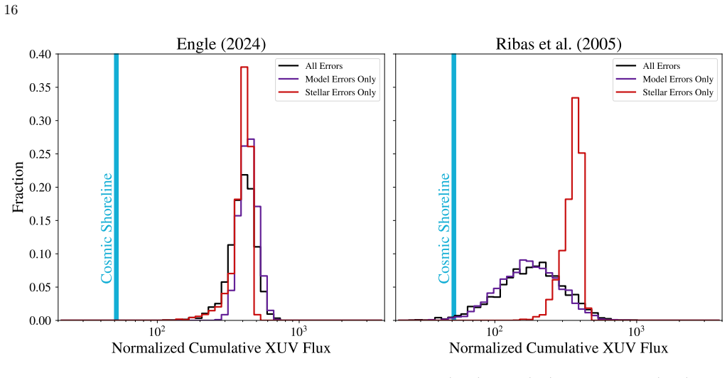
All models show GJ 1132 b has at least a 95% chance of receiving over 50 times modern Earth's XUV flux
A machine-rendered reading of the paper's core claim, the machinery that carries it, and where it could break.
Core claim
Every model permutation for the star's XUV history, including flares, gives the planet at least a 95% probability of intercepting more than 50 times the cumulative XUV flux received by modern Earth. This places GJ 1132 b firmly on the atmosphere-free side of the cosmic shoreline.
What carries the argument
The cumulative XUV flux calculation that integrates two quiescent luminosity evolution models for M dwarfs with flare contributions derived from the star's TESS light curve and Kepler statistics.
If this is right
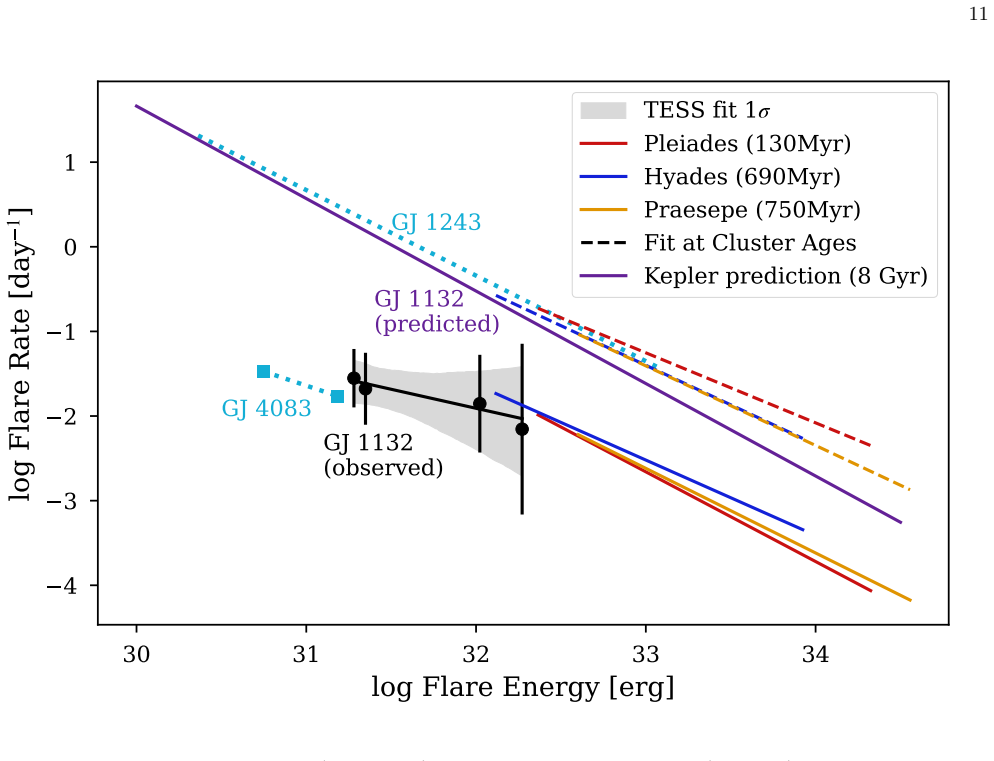
- Flares contribute about 20% of the total XUV energy delivered to the planet.
- The empirical M-dwarf XUV model predicts 2-3 times more total flux and a 2-3 times narrower distribution than the solar-twin scaling.
- GJ 1132 b lies well beyond the threshold for permanent atmospheric loss.
- Similar short-period planets around old M dwarfs are probable candidates for atmospheric stripping.
Where Pith is reading between the lines
- Atmospheric observations of GJ 1132 b could directly test the accuracy of the XUV history models.
- The result suggests that many close-in Earth-sized planets around M dwarfs may have lost their atmospheres early in their lives.
- Switching from solar-scaled to empirical M-dwarf XUV models changes predicted fluxes by a factor of 2-3 and could shift habitability assessments for other systems.
- The star's low flare rate and long rotation period are consistent with it being several Gyr old.
Load-bearing premise
The quiescent XUV luminosity evolution models accurately represent the star's history and the flare rate extrapolated from limited TESS and Kepler data applies to this system over its lifetime.
What would settle it
A direct measurement showing GJ 1132's current XUV output is much lower than the models assume, or a detection of a substantial atmosphere on GJ 1132 b, would falsify the high cumulative exposure claim.
Figures


read the original abstract
We investigate the plausible history of the XUV luminosity evolution of the planet-hosting M4 star GJ 1132 (~0.2 solar masses) to infer the cumulative incident XUV flux intercepted by the short-period (~1.6 d) Earth-sized transiting planet GJ 1132 b. We include the dominant observational uncertainties, compare two quiescent XUV luminosity evolution models, and simulate the XUV luminosity evolution from flares based on TESS data and a re-analysis of Kepler stars. We find only 4 flares in GJ 1132's TESS 123 day lightcurve, which is relatively few for M dwarfs and, in conjunction with the ~125 day period, suggests that this star is many Gyr old. We find that all model permutations predict that the planet has at least a 95% chance of receiving more than 50 times as much XUV flux as modern Earth, confirming that this planet is a good candidate for permanent atmospheric loss. We also find that an empirical XUV model for M dwarfs predicts 2-3 times more total XUV flux than a commonly used solar twin model and that the empirical model's distribution is 2-3 times narrower. Flares contribute about 20% of the cumulative XUV flux on planet b, which, while modest, ensures the planet lies firmly on the atmosphere-free side of the "cosmic shoreline."
Editorial analysis
A structured set of objections, weighed in public.
Referee Report
Summary. The manuscript models the cumulative XUV flux received by the transiting Earth-sized planet GJ 1132 b over its lifetime by combining two quiescent XUV luminosity evolution prescriptions for its ~0.2 M⊙ M4 host with flare contributions simulated from four TESS detections in 123 days plus a re-analysis of Kepler M-dwarf flare statistics. All model permutations are reported to yield at least a 95% probability that the planet has intercepted more than 50 times the modern-Earth XUV fluence, placing it firmly on the atmosphere-free side of the cosmic shoreline; flares are stated to contribute ~20% of the total while an empirical M-dwarf XUV model produces 2–3 times higher fluence than a solar-twin scaling.
Significance. If the flare-rate extrapolation and model-combination procedure are robust, the work supplies a concrete, observationally anchored probability distribution for the high-energy irradiation history of a specific rocky exoplanet, directly informing atmospheric-escape calculations and target selection for transmission spectroscopy. The quantitative comparison between empirical M-dwarf and solar-twin scalings, together with the modest but non-negligible flare term, offers a useful benchmark for similar M-dwarf systems.
major comments (2)
- [Flare modeling] Flare modeling section: the flare frequency distribution is constructed from only four TESS events and a Kepler M-dwarf sample and then integrated over the star’s full lifetime without an explicit mass-, rotation-, or age-dependent scaling. Because the quiescent models already differ by a factor of 2–3, even a modest systematic reduction in the flare rate for an old, slowly rotating 0.2 M⊙ star can shift the lower edge of the cumulative distribution relative to the 50× Earth threshold that underpins the 95% probability claim.
- [Results] Results and discussion: the statement that “all model permutations predict at least a 95% chance” is presented as the headline result, yet the manuscript does not show the sensitivity of the 5% tail to plausible variations in the flare-rate normalization or to the precise age prior inferred from the 125-day rotation period. A quantitative sensitivity table or Monte-Carlo re-sampling with varied flare scalings would be required to substantiate that the 95% threshold is stable.
minor comments (2)
- [Abstract] The abstract and introduction should explicitly name the two quiescent XUV evolution models (e.g., the specific empirical M-dwarf relation and the solar-twin scaling) rather than referring to them generically.
- [Figures] Figure captions and text should clarify how the 20% average flare contribution is computed (time-integrated fluence or instantaneous luminosity) and whether it is evaluated at the median or mean of the posterior.
Simulated Author's Rebuttal
We thank the referee for their positive evaluation of the significance of our work and for the constructive major comments on flare modeling and the robustness of our headline result. We address each point below and describe the revisions we will make to the manuscript.
read point-by-point responses
-
Referee: [Flare modeling] Flare modeling section: the flare frequency distribution is constructed from only four TESS events and a Kepler M-dwarf sample and then integrated over the star’s full lifetime without an explicit mass-, rotation-, or age-dependent scaling. Because the quiescent models already differ by a factor of 2–3, even a modest systematic reduction in the flare rate for an old, slowly rotating 0.2 M⊙ star can shift the lower edge of the cumulative distribution relative to the 50× Earth threshold that underpins the 95% probability claim.
Authors: We agree that the flare frequency distribution relies on a small number of TESS detections (four events) normalized to the Kepler M-dwarf sample and is integrated over the full stellar lifetime without an additional explicit scaling for mass, rotation rate, or age. The low observed flare rate is, however, itself consistent with the star being old and slowly rotating, as indicated by the ~125-day photometric period. The Kepler statistics supply the best available empirical shape for the FFD of M dwarfs, and our normalization is tied directly to the TESS observations of this specific star. While an age- or rotation-dependent flare scaling would be desirable, such scalings are not yet well constrained for old, low-mass M dwarfs in the literature. We will add a dedicated paragraph in the revised discussion section that explores the effect of a factor-of-two reduction in the flare contribution (a conservative adjustment for an old star) and will show that the lower edge of the cumulative XUV distribution remains above the 50× Earth threshold at high probability. revision: partial
-
Referee: [Results] Results and discussion: the statement that “all model permutations predict at least a 95% chance” is presented as the headline result, yet the manuscript does not show the sensitivity of the 5% tail to plausible variations in the flare-rate normalization or to the precise age prior inferred from the 125-day rotation period. A quantitative sensitivity table or Monte-Carlo re-sampling with varied flare scalings would be required to substantiate that the 95% threshold is stable.
Authors: The model permutations already combine the two quiescent XUV evolution prescriptions with and without the flare component. We acknowledge that an explicit sensitivity analysis of the 5 % tail to variations in flare-rate normalization and the age prior derived from the rotation period is not presented. To address this, we will add a new subsection (and accompanying table) in the revised results section that reports Monte Carlo re-samplings. These will vary the flare normalization within the Poisson uncertainty implied by four detected events and will sample the age prior over the plausible range for a 0.2 M⊙ star with a 125-day rotation period. The table will list the resulting probabilities that the cumulative XUV fluence exceeds 50 times the modern-Earth value, thereby demonstrating the stability of the 95 % threshold under these variations. revision: yes
Circularity Check
No circularity: external models integrated with direct observations
full rationale
The derivation integrates two literature quiescent XUV evolution models with a flare simulation built from the paper's own TESS light curve (4 flares in 123 days) plus a re-analysis of independent Kepler M-dwarf data. Cumulative flux and the 95% probability threshold are computed forward from these inputs; no equation redefines a fitted quantity as its own prediction, no ansatz is smuggled via self-citation, and the central claim does not reduce to a renaming or self-definition. The result remains falsifiable against external stellar-age and flare-rate benchmarks.
Axiom & Free-Parameter Ledger
free parameters (2)
- quiescent XUV luminosity evolution parameters
- flare rate and contribution parameters
axioms (2)
- domain assumption The star's age inferred from low flare rate and ~125 day period
- domain assumption Applicability of Kepler flare statistics to GJ 1132 over its lifetime
Reference graph
Works this paper leans on
-
[1]
Astropy Collaboration, Price-Whelan, A. M., Lim, P. L., et al. 2022,Astrophys. J., 935, 167, doi: 10.3847/1538-4357/ac7c74
-
[2]
Baraffe, I., Homeier, D., Allard, F., & Chabrier, G. 2015, Astron. & Astrophys., 577, A42, doi: 10.1051/0004-6361/201425481
-
[3]
2020, PASP, 132, 024502, doi: 10.1088/1538-3873/ab3ce8
Barnes, R., Luger, R., Deitrick, R., et al. 2020, Publications of the Astronomical Society of the Pacific, 132, 024502, doi: 10.1088/1538-3873/ab3ce8
-
[4]
K., Wachiraphan, P., & Murray, C
Berta-Thompson, Z. K., Wachiraphan, P., & Murray, C. 2025, arXiv e-prints, arXiv:2507.02136, doi: 10.48550/arXiv.2507.02136
-
[5]
K., Irwin, J., Charbonneau, D., et al
Berta-Thompson, Z. K., Irwin, J., Charbonneau, D., et al. 2015,Nature, 527, 204, doi: 10.1038/nature15762
-
[6]
Bidelman, W. P. 1985,Astrophys. J. Supp., 59, 197, doi: 10.1086/191069
-
[7]
2026,Proc
Birky, J., & Barnes, R. 2026,Proc. Astron. Soc. Pac
2026
-
[8]
Birky, J., Barnes, R., & Davenport, J. R. A. 2025, Astrophys. J., 992, 133, doi: 10.3847/1538-4357/adf4cf 18
-
[9]
Birky, J., Barnes, R., & Fleming, D. P. 2021, Research Notes of the American Astronomical Society, 5, 122, doi: 10.3847/2515-5172/ac034c
-
[10]
Bonfils, X., Almenara, J. M., Cloutier, R., et al. 2018, Astron. & Astrophys., 618, A142, doi: 10.1051/0004-6361/201731884
-
[11]
2019, PASP, 131, 108005, doi: 10.1088/1538-3873/aae7fc —
Buchner, J. 2019,Proc. Astron. Soc. Pac., 131, 108005, doi: 10.1088/1538-3873/aae7fc —. 2021, The Journal of Open Source Software, 6, 3001, doi: 10.21105/joss.03001
-
[12]
Buchner, J., Georgakakis, A., Nandra, K., et al. 2014, Astron. & Astrophys., 564, A125, doi: 10.1051/0004-6361/201322971
-
[13]
SIAM Journal on Scientific Computing 16(5):1190--1208
Byrd, R. H., Lu, P., Nocedal, J., & Zhu, C. 1995, SIAM Journal on Scientific Computing, 16, 1190, doi: 10.1137/0916069
-
[14]
R., Tasse, C., Keers, R., et al
Callingham, J. R., Tasse, C., Keers, R., et al. 2025,Nature, 647, 603, doi: 10.1038/s41586-025-09715-3
-
[15]
Chatterjee, R. D., & Pierrehumbert, R. T. 2026, Astrophys. J., 998, 236, doi: 10.3847/1538-4357/ae2ffa
-
[16]
Crossfield, I. J. M., Malik, M., Hill, M. L., et al. 2022, Astrophys. J. Lett., 937, L17, doi: 10.3847/2041-8213/ac886b
-
[17]
Davenport, J. R. A., Covey, K. R., Clarke, R. W., et al. 2019,Astrophys. J., 871, 241, doi: 10.3847/1538-4357/aafb76
-
[18]
Davenport, J. R. A., Mendoza, G. T., & Hawley, S. L. 2020,Astron. J., 160, 36, doi: 10.3847/1538-3881/ab9536
-
[19]
Davenport, J. R. A., Hawley, S. L., Hebb, L., et al. 2014, Astrophys. J., 797, 122, doi: 10.1088/0004-637X/797/2/122 do Amaral, L. N. R., Barnes, R., Segura, A., & Luger, R. 2022,Astrophys. J., 928, 12, doi: 10.3847/1538-4357/ac53af
-
[20]
2013,Icarus, 226, 1447, doi: 10.1016/j.icarus.2013.07.025
Driscoll, P., & Bercovici, D. 2013,Icarus, 226, 1447, doi: 10.1016/j.icarus.2013.07.025
-
[21]
Driscoll, P. E., & Barnes, R. 2015, Astrobiology, 15, 739, doi: 10.1089/ast.2015.1325
-
[22]
Engle, S. G. 2024,Astrophys. J., 960, 62, doi: 10.3847/1538-4357/ad0840
-
[23]
Engle, S. G., & Guinan, E. F. 2023,Astrophys. J. Lett., 954, L50, doi: 10.3847/2041-8213/acf472
-
[24]
Feinstein, A. D., Montet, B. T., Ansdell, M., et al. 2020, Astron. J., 160, 219, doi: 10.3847/1538-3881/abac0a
-
[25]
Feroz, F., Hobson, M. P., & Bridges, M. 2009, Mon. Not. R. Astron. Soc., 398, 1601, doi: 10.1111/j.1365-2966.2009.14548.x
-
[26]
Feroz, F., Hobson, M. P., Cameron, E., & Pettitt, A. N. 2019, The Open Journal of Astrophysics, 2, 10, doi: 10.21105/astro.1306.2144
-
[27]
P., Barnes, R., Luger, R., & VanderPlas, J
Fleming, D. P., Barnes, R., Luger, R., & VanderPlas, J. T. 2020,Astrophys. J., 891, 155, doi: 10.3847/1538-4357/ab77ad
-
[28]
J., & Driscoll, P
Foley, B. J., & Driscoll, P. E. 2016, Geochemistry,
2016
-
[29]
Geophysics, Geosystems, 17, 1885, doi: 10.1002/2015GC006210
-
[30]
Foreman-Mackey, D., Hogg, D. W., Lang, D., & Goodman, J. 2013,Proc. Astron. Soc. Pac., 125, 306, doi: 10.1086/670067
-
[31]
France, K., Duvvuri, G., Froning, C. S., et al. 2025, Astron. J., 170, 159, doi: 10.3847/1538-3881/adefdf
-
[32]
2026,Plan
Gialluca, M. 2026,Plan. Sci. J
2026
-
[33]
Gialluca, M. T., Barnes, R., Meadows, V. S., et al. 2024, Plan. Sci. J., 5, 137, doi: 10.3847/PSJ/ad4454
-
[34]
2010, CAMCS, 5, 65, doi: 10.2140/camcos.2010.5.65
Goodman, J., & Weare, J. 2010, Communications in Applied Mathematics and Computational Science, 5, 65, doi: 10.2140/camcos.2010.5.65
-
[35]
Gunell, H., Maggiolo, R., Nilsson, H., et al. 2018, Astron. & Astrophys., 614, L3, doi: 10.1051/0004-6361/201832934 G¨ unther, M. N., Zhan, Z., Seager, S., et al. 2020, Astron. J., 159, 60, doi: 10.3847/1538-3881/ab5d3a
-
[36]
Handley, W. J., Hobson, M. P., & Lasenby, A. N. 2015a, Mon. Not. R. Astron. Soc., 453, 4384, doi: 10.1093/mnras/stv1911 —. 2015b,Mon. Not. R. Astron. Soc., 450, L61, doi: 10.1093/mnrasl/slv047
-
[37]
Harris, C. R., Oliphant, T. E., Virtanen, P., et al. 2020, Nature, 585, 357, doi: 10.1038/s41586-020-2649-2
-
[38]
<i>KEPLER</i>FLARES. I. ACTIVE AND INACTIVE M DWARFS
Hawley, S. L., Davenport, J. R. A., Kowalski, A. F., et al. 2014,Astrophys. J., 797, 121, doi: 10.1088/0004-637X/797/2/121
-
[39]
Statistics and Computing , keywords =
Higson, E., Handley, W., Hobson, M., & Lasenby, A. 2019, Statistics and Computing, 29, 891, doi: 10.1007/s11222-018-9844-0
-
[40]
Hunt-Walker, N. M., Hilton, E. J., Kowalski, A. F., Hawley, S. L., & Matthews, J. M. 2012,Proc. Astron. Soc. Pac., 124, 545, doi: 10.1086/666495
-
[41]
Hunter, J. D. 2007, Computing In Science & Engineering, 9, 90
2007
-
[42]
M.-R., Diamond-Lowe, H., et al
Ih, J., Kempton, E. M.-R., Diamond-Lowe, H., et al. 2025, arXiv e-prints, arXiv:2508.08253, doi: 10.48550/arXiv.2508.08253
-
[43]
doi:10.1051/0004-6361/201834400 , keywords =
Ilin, E., Schmidt, S. J., Davenport, J. R. A., & Strassmeier, K. G. 2019,Astron. & Astrophys., 622, A133, doi: 10.1051/0004-6361/201834400
-
[44]
doi:10.1051/0004-6361/202039198 , keywords =
Ilin, E., Schmidt, S. J., Poppenh¨ ager, K., et al. 2021, Astron. & Astrophys., 645, A42, doi: 10.1051/0004-6361/202039198 19
-
[45]
M., et al., 2016, in Chiozzi G., Guzman J
Jenkins, J. M., Twicken, J. D., McCauliff, S., et al. 2016, Proc. SPIE, 9913, 99133E, doi: 10.1117/12.2233418
-
[46]
Ji, X., Chatterjee, R. D., Coy, B. P., & Kite, E. 2025, Astrophys. J., 992, 198, doi: 10.3847/1538-4357/adfe69
-
[47]
2015, Bayesian Active Learning for Posterior Estimation
Kandasamy, K., Schneider, J., & Poczos, B. 2015, Bayesian Active Learning for Posterior Estimation
2015
-
[48]
2017, Artificial Intelligence, 243, 45, doi: 10.1016/j.artint.2016.11.002
Kandasamy, K., Schneider, J., & P´ oczos, B. 2017, Artificial Intelligence, 243, 45, doi: 10.1016/j.artint.2016.11.002
-
[49]
Kreidberg, L., Koll, D. D. B., Morley, C., et al. 2019, Nature, 573, 87, doi: 10.1038/s41586-019-1497-4
-
[50]
Krissansen-Totton, J., & Fortney, J. J. 2022,Astrophys. J., 933, 115, doi: 10.3847/1538-4357/ac69cb
-
[51]
Lee, E. J., & Owen, J. E. 2025,Astrophys. J. Lett., 980, L40, doi: 10.3847/2041-8213/adafa3 Lightkurve Collaboration, Cardoso, J. V. d. M., Hedges, C., et al. 2018, Lightkurve: Kepler and TESS time series analysis in Python, Astrophysics Source Code Library, ascl:1812.013. https://docs.lightkurve.org
-
[52]
Loyd, R. O. P., Shkolnik, E. L., Schneider, A. C., et al. 2018,Astrophys. J., 867, 70, doi: 10.3847/1538-4357/aae2ae
-
[53]
2015, Astrobiology, 15, 119, doi: 10.1089/ast.2014.1231 Mat´ ern, B
Luger, R., & Barnes, R. 2015, Astrobiology, 15, 119, doi: 10.1089/ast.2014.1231 Mat´ ern, B. 1986, Lecture Notes in Statistics, Vol. 36, Spatial Variation, 2nd edn. (New York: Springer), doi: 10.1007/978-1-4615-7892-5
-
[54]
McGovern, P. J., & Schubert, G. 1989, Earth and Planetary Science Letters, 96, 27, doi: 10.1016/0012-821X(89)90121-0 Morales-Calder´ on, M., Joyce, S. R. G., Pye, J. P., et al. 2024,Astron. & Astrophys., 688, A45, doi: 10.1051/0004-6361/202449832
-
[55]
Mordasini, C. 2020,Astron. & Astrophys., 638, A52, doi: 10.1051/0004-6361/201935541
-
[56]
2006, Earth Planet
Olson, P., & Christensen, U. 2006, Earth Planet. Sci. Lett., 250, 561
2006
-
[57]
A., & Wolk, S
Osten, R. A., & Wolk, S. J. 2015, The Astrophysical Journal, 809, 79
2015
-
[58]
K., Charbonneau, D., & Vanderburg, A
Pass, E. K., Charbonneau, D., & Vanderburg, A. 2025, Astrophys. J. Lett., 986, L3, doi: 10.3847/2041-8213/adda39
-
[59]
Peacock, S., Barman, T., Shkolnik, E. L., Hauschildt, P. H., & Baron, E. 2019,Astrophys. J., 871, 235, doi: 10.3847/1538-4357/aaf891
-
[60]
Peacock, S., Wilson, D. J., Richey-Yowell, T., et al. 2025, Astron. J., 170, 293, doi: 10.3847/1538-3881/ae0a2f
-
[61]
E., & Williams, C
Rasmussen, C. E., & Williams, C. K. I. 2006, Gaussian Processes for Machine Learning (Cambridge, MA: The MIT Press)
2006
-
[62]
Ribas, I., Guinan, E. F., G¨ udel, M., & Audard, M. 2005, Astrophys. J., 622, 680, doi: 10.1086/427977
-
[63]
Richey-Yowell, T., Shkolnik, E. L., Loyd, R. O. P., et al. 2022,Astrophys. J., 929, 169, doi: 10.3847/1538-4357/ac5f48
-
[64]
Rousseeuw, P. J., & Croux, C. 1993, Journal of the American Statistical Association, 88, 1273, doi: 10.1080/01621459.1993.10476408
-
[65]
Astronomy & Astrophysics , author =
Sanz-Forcada, J., L´ opez-Puertas, M., Lamp´ on, M., et al. 2025,Astron. & Astrophys., 693, A285, doi: 10.1051/0004-6361/202451680
-
[66]
Savitzky, A., & Golay, M. J. E. 1964, Analytical Chemistry, 36, 1627, doi: 10.1021/ac60214a047
-
[67]
Schneider, A. C., & Shkolnik, E. L. 2018,Astron. J., 155, 122, doi: 10.3847/1538-3881/aaaa24
-
[68]
Skilling, J. 2004, in AIP Conference Proceedings, Vol. 735, Bayesian Inference and Maximum Entropy Methods in Science and Engineering: 24th International Workshop, 395–405, doi: 10.1063/1.1835238
-
[69]
Speagle, J. S. 2020,Mon. Not. R. Astron. Soc., 493, 3132, doi: 10.1093/mnras/staa278
-
[70]
Storn, R., & Price, K. 1997, Journal of Global Optimization, 11, 341, doi: 10.1023/A:1008202821328
-
[71]
Virtanen, P., Gommers, R., Oliphant, T. E., et al. 2020, Nature Methods, 17, 261, doi: 10.1038/s41592-019-0686-2
-
[72]
Wachiraphan, P., Berta-Thompson, Z. K., Diamond-Lowe, H., et al. 2025,Astron. J., 169, 311, doi: 10.3847/1538-3881/adc990
-
[73]
Wang, H., & Li, J. 2018, Neural Computation, 30, 3072, doi: 10.1162/neco a 01127 Weiner Mansfield, M., Xue, Q., Zhang, M., et al. 2024, Astrophys. J. Lett., 975, L22, doi: 10.3847/2041-8213/ad8161
-
[74]
Xue, Q., Bean, J. L., Zhang, M., et al. 2024, arXiv e-prints, arXiv:2408.13340, doi: 10.48550/arXiv.2408.13340
-
[75]
B., & Kasting, J
Zahnle, K., Pollack, J. B., & Kasting, J. F. 1990, Icarus, 84, 502
1990
-
[76]
Zahnle, K. J., & Catling, D. C. 2017,Astrophys. J., 843, 122, doi: 10.3847/1538-4357/aa7846 20 APPENDIX A.ALABI KERNEL AND SCALING Bayesian inference requires evaluating the likelihood function at thousands to millions of points in parameter space. When each likelihood evaluation demands a forward-model simulation that takes seconds to minutes, direct sam...
discussion (0)
Sign in with ORCID, Apple, or X to comment. Anyone can read and Pith papers without signing in.