Recognition: unknown
Stability and Bifurcation Analysis of Fractional Delay Differential Equation with a Delay-dependent Coefficient
Pith reviewed 2026-05-08 16:30 UTC · model grok-4.3
The pith
A general stability result for fractional delay equations with two delays holds for every fractional order and any positive first delay.
A machine-rendered reading of the paper's core claim, the machinery that carries it, and where it could break.
Core claim
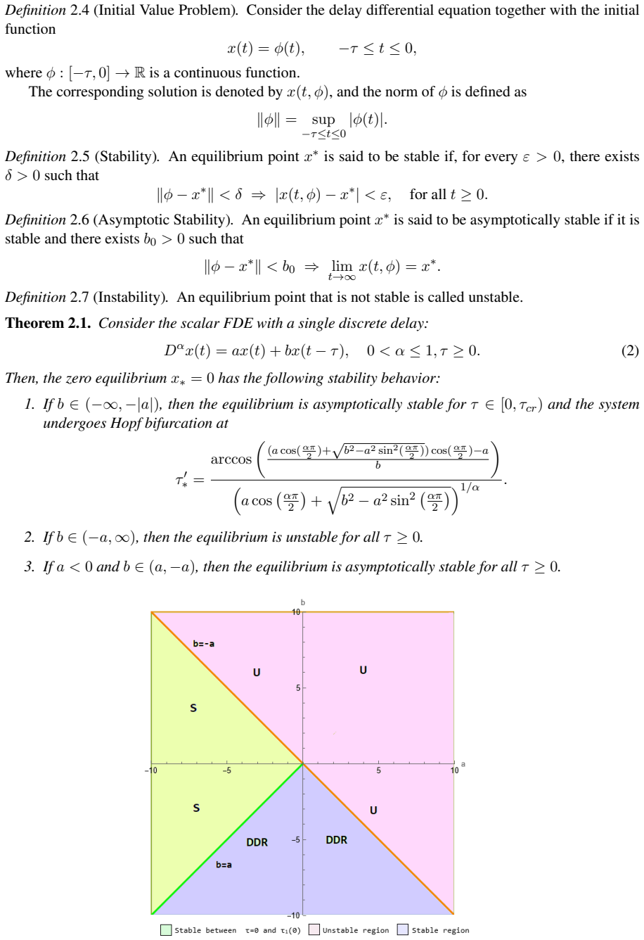
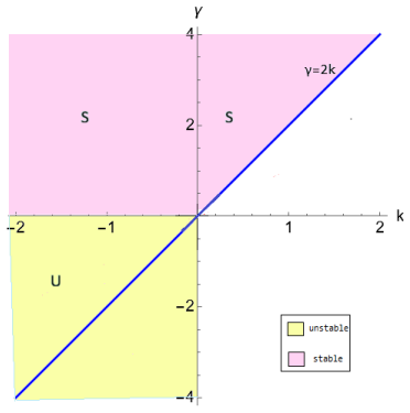
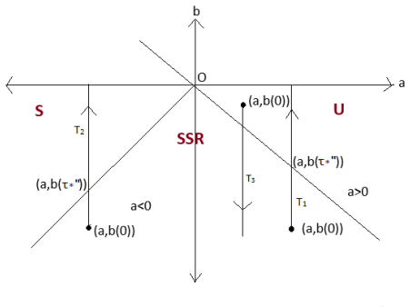
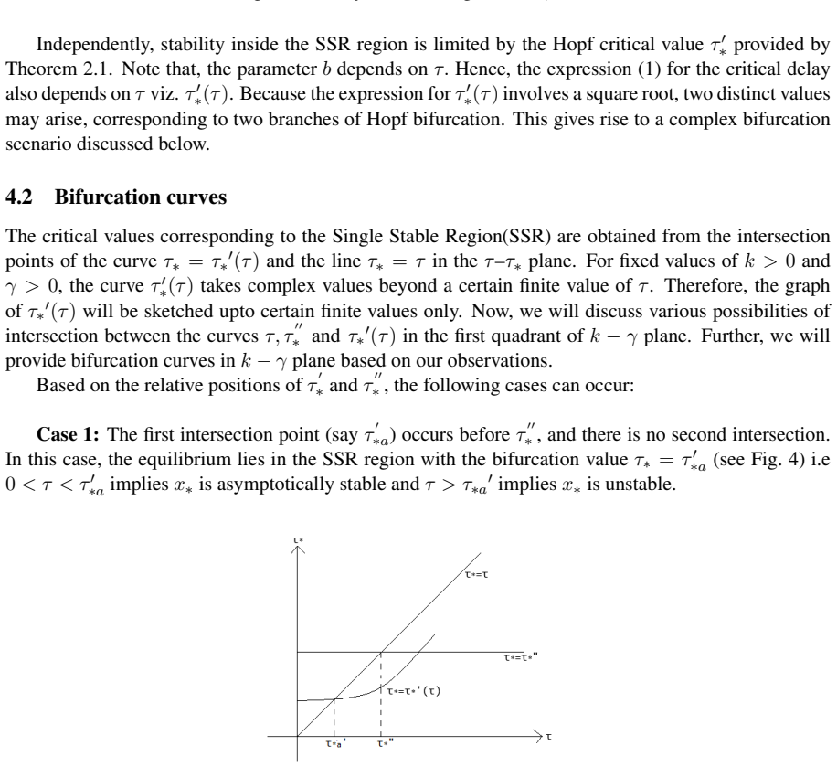
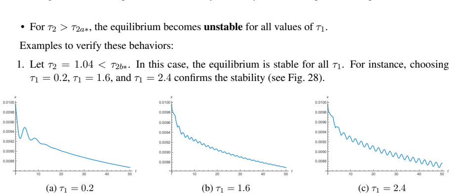
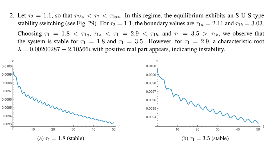
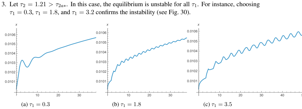
For the linearized system corresponding to the given fractional delay equation with τ1 > 0 and τ2 ≥ 0, the stability criteria in the (k, γ) plane hold for all fractional orders 0 < α ≤ 1 and all positive values of τ1. This general result is illustrated through stability diagrams in the (τ1, τ2) plane obtained via numerical methods for fixed parameter values.
What carries the argument
The characteristic equation arising from linearization of the fractional delay equation around the zero solution, using the slope k = g'(0) at the origin to determine stability switches and Hopf bifurcation points.
If this is right
- Stability boundaries in the (k, γ) plane can be determined explicitly for the reduced case τ1 = 0.
- Stability regions in the two-delay plane can be mapped numerically for any chosen fractional order, k, and γ.
- The general result implies that changing the fractional order does not move the stability boundaries when both delays are positive.
- Bifurcation curves separate stable and unstable regions and can be tracked as delays vary.
Where Pith is reading between the lines
- The independence from α suggests the same stability diagrams may apply when approximating fractional systems by high-order integer-order equations.
- The form of the delay-dependent coefficient may arise in other models with signal attenuation over a second delay interval.
- Extending the linear analysis to specific nonlinear g functions would test whether the stability regions persist beyond the local approximation.
Load-bearing premise
The analysis assumes linearization around the trivial equilibrium via the derivative k = g'(0) and that fractional-order stability criteria apply directly to the resulting characteristic equation.
What would settle it
A numerical integration or eigenvalue computation for specific α, k, γ, and positive τ1, τ2 that shows the stability boundary in the (τ1, τ2) plane crossing a point predicted to be stable by the general result would falsify the claim.
Figures


read the original abstract
This paper investigates the stability of different regions in the $(k,\gamma)$-plane for a class of fractional delay differential equations given by \begin{equation} D^{\alpha} x(t) = -\gamma x(t) + g\big(x(t - \tau_1)\big) - e^{-\gamma \tau_2}\, g\big(x(t - \tau_1 - \tau_2)\big), \qquad 0 < \alpha \le 1, \end{equation} where $k = g'(0)$. The primary focus is on the stability of the trivial equilibrium of the corresponding linearized system. A detailed stability and bifurcation analysis is carried out for the particular case $\tau_1 = 0$ and $\tau_2 \ge 0$. Furthermore, a general result is established for the case $\tau_1 > 0$, $\tau_2 \ge 0$, which holds for all values of $\alpha$ and $\tau_1$. In addition, illustrative examples are provided in the form of stability diagrams in the $(\tau_1,\tau_2)$-plane for fixed values of $\alpha$, $k$, and $\gamma$. These diagrams are generated using appropriate numerical methods to visualize the stability regions and to support the theoretical results.
Editorial analysis
A structured set of objections, weighed in public.
Referee Report
Summary. The manuscript analyzes stability and bifurcations of the trivial equilibrium for the fractional DDE D^α x(t) = -γ x(t) + g(x(t-τ1)) - e^{-γ τ2} g(x(t-τ1-τ2)) with 0<α≤1. Detailed stability regions in the (k,γ)-plane are derived for the special case τ1=0, τ2≥0. A general stability result is asserted for τ1>0, τ2≥0 that is claimed to hold for every α in (0,1] and every τ1. Numerical stability diagrams in the (τ1,τ2)-plane are generated for fixed α, k, γ to illustrate the regions.
Significance. If the general result is rigorously established, the work would be significant for fractional-order delay systems: it would identify a structural feature (the specific combination of delayed terms with the exponential coefficient) that renders stability regions independent of α, which is atypical and could simplify analysis in applications such as control or population models. The numerical diagrams provide concrete support for fixed-α cases, though their value is reduced by the lack of α-variation testing.
major comments (2)
- [General result for τ1 > 0] The section establishing the general result for τ1>0, τ2≥0: the claim that the result holds for all 0<α≤1 rests on the characteristic equation s^α + γ - k e^{-s τ1} + k e^{-γ τ2} e^{-s(τ1+τ2)}=0. Standard DDE crossing criteria (pure imaginary roots, Routh-Hurwitz on the quasi-polynomial) are derived under Re(s)=0, but fractional-order stability requires |arg(s)| > α π/2. No explicit argument is given showing that the stability boundary or crossing conditions are invariant under changes in α, nor is it shown that roots cannot enter the unstable sector for α<1 while remaining stable for α=1. This directly undermines the universality assertion, which is load-bearing for the central claim.
- [Numerical examples] Numerical examples section: the stability diagrams are produced only for fixed values of α. While they illustrate the (τ1,τ2) regions for those specific α, they provide no test of the α-independence asserted in the general result; a single diagram varying α (or an analytic proof that the boundary curves do not move) is needed to support the claim.
minor comments (2)
- [Abstract] The abstract and introduction should explicitly state the precise form of the general result (e.g., the explicit stability condition in the (k,γ) or (τ1,τ2) plane) rather than referring only to its existence.
- [Linearization] Notation for the linearized coefficient k = g'(0) is introduced without a dedicated equation number; adding an equation label would improve traceability when the characteristic equation is later written.
Simulated Author's Rebuttal
We thank the referee for the thorough review and valuable feedback on our manuscript. The comments have helped us identify areas where the presentation of the general stability result and its numerical support can be strengthened. We address each major comment below and outline the revisions we will make.
read point-by-point responses
-
Referee: [General result for τ1 > 0] The section establishing the general result for τ1>0, τ2≥0: the claim that the result holds for all 0<α≤1 rests on the characteristic equation s^α + γ - k e^{-s τ1} + k e^{-γ τ2} e^{-s(τ1+τ2)}=0. Standard DDE crossing criteria (pure imaginary roots, Routh-Hurwitz on the quasi-polynomial) are derived under Re(s)=0, but fractional-order stability requires |arg(s)| > α π/2. No explicit argument is given showing that the stability boundary or crossing conditions are invariant under changes in α, nor is it shown that roots cannot enter the unstable sector for α<1 while remaining stable for α=1. This directly undermines the universality assertion, which is load-bearing for the central claim.
Authors: We agree that an explicit demonstration of α-invariance is necessary to rigorously support the general result. The specific structure of the system, with the delay-dependent coefficient e^{-γ τ2} multiplying the second delayed term, leads to a characteristic equation whose stability boundaries in the (k, γ) and (τ1, τ2) planes are determined by magnitude and frequency conditions that coincide for all α ∈ (0,1]. In particular, substituting s = iω into the equation and separating real and imaginary parts yields crossing conditions independent of the fractional order because the exponential prefactor compensates for the argument shift introduced by s^α. We acknowledge that this reasoning was not spelled out in sufficient detail. In the revised manuscript we will insert a new subsection immediately following the derivation of the characteristic equation that explicitly derives the Hopf crossing conditions for general α, shows that the critical curves remain unchanged, and confirms that no additional unstable roots enter the sector |arg(s)| < απ/2 for α < 1. revision: yes
-
Referee: [Numerical examples] Numerical examples section: the stability diagrams are produced only for fixed values of α. While they illustrate the (τ1,τ2) regions for those specific α, they provide no test of the α-independence asserted in the general result; a single diagram varying α (or an analytic proof that the boundary curves do not move) is needed to support the claim.
Authors: We concur that numerical confirmation across α values would provide useful supporting evidence. In the revised version we will augment the numerical examples section with an additional figure that overlays stability boundaries in the (τ1, τ2)-plane for three representative fractional orders (α = 0.5, 0.8, and 1.0) at the same fixed k and γ. This will visually demonstrate that the curves coincide, thereby corroborating the analytic claim of α-independence. If space constraints arise, we will instead include a short table of critical (τ1, τ2) pairs computed for multiple α values to illustrate the invariance. revision: yes
Circularity Check
No circularity: derivation from linearized fractional DDE characteristic equation is self-contained.
full rationale
The paper starts from the given fractional DDE, linearizes around the trivial equilibrium to obtain the characteristic equation involving s^α, and applies stability analysis for the cases τ1=0 and τ1>0. No parameters are fitted to produce the claimed stability regions, no self-citation chain justifies the core result, and the general claim for all α is presented as following from the model equations rather than being redefined by them. Numerical diagrams are illustrative only. The derivation chain does not reduce to its inputs by construction.
Axiom & Free-Parameter Ledger
axioms (2)
- standard math The fractional derivative operator D^α satisfies standard properties for 0 < α ≤ 1.
- domain assumption The function g is continuously differentiable at zero so that k = g'(0) is well-defined.
Reference graph
Works this paper leans on
-
[1]
Igor Podlubny.Fractional differential equations: An introduction to fractional derivatives, frac- tional differential equations, to methods of their solution and some of their applications, volume
-
[2]
Elsevier, 2006
Anatoli ˘ı Aleksandrovich Kilbas, Hari M Srivastava, and Juan J Trujillo.Theory and applications of fractional differential equations, volume 204. Elsevier, 2006
2006
-
[3]
The analysis of fractional differential equations.Lecture notes in mathematics, 2004, 2010
Kai Diethelm and NJ Ford. The analysis of fractional differential equations.Lecture notes in mathematics, 2004, 2010
2004
-
[4]
Keith B Oldham. J. spanier the fractional calculus.Mathematics in Science and Engineering, 111, 1974
1974
-
[5]
World Scientific, 2022
Francesco Mainardi.Fractional calculus and waves in linear viscoelasticity: an introduction to mathematical models. World Scientific, 2022
2022
-
[6]
A theoretical basis for the application of fractional calculus to viscoelasticity.Journal of Rheology, 27(3):201–210, 1983
Ronald L Bagley and Peter J Torvik. A theoretical basis for the application of fractional calculus to viscoelasticity.Journal of Rheology, 27(3):201–210, 1983
1983
-
[7]
Academic Press, San Diego, 1999
Igor Podlubny.Fractional Differential Equations. Academic Press, San Diego, 1999
1999
-
[8]
Stability of caputo fractional differential equations with non-instantaneous impulses.Commun
RA VI Agarwal, D O’Regan, and S Hristova. Stability of caputo fractional differential equations with non-instantaneous impulses.Commun. Appl. Anal, 20:149–174, 2016
2016
-
[9]
Springer Science & Business Media, 2013
Jack K Hale and Sjoerd M Verduyn Lunel.Introduction to functional differential equations, vol- ume 99. Springer Science & Business Media, 2013
2013
-
[10]
Springer, 2009
Thomas Erneux.Applied delay differential equations. Springer, 2009
2009
-
[11]
Academic press, 1993
Yang Kuang.Delay differential equations: with applications in population dynamics, volume 191. Academic press, 1993
1993
-
[12]
A simple chaotic delay differential equation.Physics Letters A, 366(4-5):397–402, 2007
JC Sprott. A simple chaotic delay differential equation.Physics Letters A, 366(4-5):397–402, 2007
2007
-
[13]
Chaos in delay differential equations with applications in population dy- namics.Discrete Contin
Alfonso Ruiz-Herrera. Chaos in delay differential equations with applications in population dy- namics.Discrete Contin. Dyn. Syst, 33(4):1633–1644, 2013
2013
-
[14]
Springer Science & Business Media, 2011
Tam ´as Insperger and G ´abor St´ep´an.Semi-discretization for time-delay systems: stability and en- gineering applications, volume 178. Springer Science & Business Media, 2011
2011
-
[15]
Control design for time-delay systems based on quasi-direct pole placement.Journal of Process Control, 20(3):337–343, 2010
Wim Michiels, Tom ´aˇs Vyhl´ıdal, and Pavel Z´ıtek. Control design for time-delay systems based on quasi-direct pole placement.Journal of Process Control, 20(3):337–343, 2010
2010
-
[16]
Computer aided control system design for time delay systems using matlab®
Suat Gumussoy and Pascal Gahinet. Computer aided control system design for time delay systems using matlab®. InDelay Systems: From Theory to Numerics and Applications, pages 257–270. Springer, 2014
2014
-
[17]
CRC Press, 2000
Ravi P Agarwal.Difference equations and inequalities: theory, methods, and applications. CRC Press, 2000
2000
-
[18]
A predictor-corrector scheme for solving nonlinear delay differential equations of fractional order.J
Sachin Bhalekar and Varsha Daftardar-Gejji. A predictor-corrector scheme for solving nonlinear delay differential equations of fractional order.J. Fract. Calc. Appl, 1(5):1–9, 2011
2011
-
[19]
A new predictor–corrector method for fractional differential equations.Applied Mathematics and Computation, 244:158–182, 2014
Varsha Daftardar-Gejji, Yogita Sukale, and Sachin Bhalekar. A new predictor–corrector method for fractional differential equations.Applied Mathematics and Computation, 244:158–182, 2014. 22
2014
-
[20]
Stability and bifurcation analysis of a generalized scalar delay differential equa- tion.Chaos: An Interdisciplinary Journal of Nonlinear Science, 26(8), 2016
Sachin Bhalekar. Stability and bifurcation analysis of a generalized scalar delay differential equa- tion.Chaos: An Interdisciplinary Journal of Nonlinear Science, 26(8), 2016
2016
-
[21]
Fractional bloch equation with delay.Computers & Mathematics with Applications, 61(5):1355–1365, 2011
Sachin Bhalekar, Varsha Daftardar-Gejji, Dumitru Baleanu, and Richard Magin. Fractional bloch equation with delay.Computers & Mathematics with Applications, 61(5):1355–1365, 2011
2011
-
[22]
Fractional order sunflower equation: stability, bifurcation and chaos.The European Physical Journal Special Topics, pages 1–11, 2024
Deepa Gupta and Sachin Bhalekar. Fractional order sunflower equation: stability, bifurcation and chaos.The European Physical Journal Special Topics, pages 1–11, 2024
2024
-
[23]
Stability and bifurcation analysis of a fractional order delay differential equation involving cubic nonlinearity.Chaos, Solitons & Fractals, 162:112483, 2022
Sachin Bhalekar and Deepa Gupta. Stability and bifurcation analysis of a fractional order delay differential equation involving cubic nonlinearity.Chaos, Solitons & Fractals, 162:112483, 2022
2022
-
[24]
Practical stability for riemann–liouville delay fractional differential equations.Arabian Journal of Mathematics, 10(2):271–283, 2021
Ravi Agarwal, Snezhana Hristova, and Donal O’Regan. Practical stability for riemann–liouville delay fractional differential equations.Arabian Journal of Mathematics, 10(2):271–283, 2021
2021
-
[25]
Generalized proportional caputo fractional differential equations with delay and practical stability by the razumikhin method.Mathematics, 10(11):1849, 2022
Ravi Agarwal, Snezhana Hristova, and Donal O’Regan. Generalized proportional caputo fractional differential equations with delay and practical stability by the razumikhin method.Mathematics, 10(11):1849, 2022
2022
-
[26]
Dynamical analysis of fractional order uc ¸ar prototype delayed system.Signal, Image and Video Processing, 6(3):513–519, 2012
Sachin Bhalekar. Dynamical analysis of fractional order uc ¸ar prototype delayed system.Signal, Image and Video Processing, 6(3):513–519, 2012
2012
-
[27]
Dynamics of fractional-ordered Chen system with delay.Pramana, 79:61–69, 2012
Varsha Daftardar-Gejji, Sachin Bhalekar, and Prashant Gade. Dynamics of fractional-ordered Chen system with delay.Pramana, 79:61–69, 2012
2012
-
[28]
Springer Science & Business Media, 2003
Keqin Gu, Jie Chen, and Vladimir L Kharitonov.Stability of time-delay systems. Springer Science & Business Media, 2003
2003
-
[29]
Springer, 2002
Silviu-Iulian Niculescu.Delay effects on stability: a robust control approach. Springer, 2002
2002
-
[30]
On a two lag differential delay equation.The ANZIAM Journal, 24(3):292–317, 1983
RD Braddock and P Van den Driessche. On a two lag differential delay equation.The ANZIAM Journal, 24(3):292–317, 1983
1983
-
[31]
Hopf bifurcation in a solid avascular tumour growth model with two discrete delays.Mathematical and Computer Modelling, 47(5-6):597–603, 2008
Monika Joanna Piotrowska. Hopf bifurcation in a solid avascular tumour growth model with two discrete delays.Mathematical and Computer Modelling, 47(5-6):597–603, 2008
2008
-
[32]
Stability analysis of an equation with two delays and application to the production of platelets.Discrete and Continuous Dynamical Systems-Series S, 13(11):3005–3027, 2020
Lo ¨ıs Boullu, Laurent Pujo-Menjouet, and Jacques B ´elair. Stability analysis of an equation with two delays and application to the production of platelets.Discrete and Continuous Dynamical Systems-Series S, 13(11):3005–3027, 2020
2020
-
[33]
Geometric stability switch criteria in delay differential equations with two delays and delay dependent parameters
Qi An, Edoardo Beretta, Yang Kuang, Chuncheng Wang, and Hao Wang. Geometric stability switch criteria in delay differential equations with two delays and delay dependent parameters. Journal of Differential Equations, 266(11):7073–7100, 2019
2019
-
[34]
Chengming Huang and Stefan Vandewalle. An analysis of delay-dependent stability for ordinary and partial differential equations with fixed and distributed delays.SIAM Journal on Scientific Computing, 25(5):1608–1632, 2004
2004
-
[35]
Delay dependent stability of highly nonlinear hybrid stochastic systems.Automatica, 82:165–170, 2017
Weiyin Fei, Liangjian Hu, Xuerong Mao, and Mingxuan Shen. Delay dependent stability of highly nonlinear hybrid stochastic systems.Automatica, 82:165–170, 2017
2017
-
[36]
Pragati Dutta and Sachin Bhalekar. Some stability results for the fractional differential equations with two delays.arXiv preprint arXiv:2509.21937, 2025
-
[37]
Springer Science & Business Media, 2011
Muthusamy Lakshmanan and Dharmapuri Vijayan Senthilkumar.Dynamics of nonlinear time- delay systems. Springer Science & Business Media, 2011
2011
-
[38]
springer, 2010
Hal L Smith.An introduction to delay differential equations with applications to the life sciences. springer, 2010. 23
2010
discussion (0)
Sign in with ORCID, Apple, or X to comment. Anyone can read and Pith papers without signing in.