Recognition: unknown
Marking strategies for adaptive mesh refinement: An efficiency-focused benchmark study for steady solid and fluid mechanics problems
Pith reviewed 2026-05-09 20:30 UTC · model grok-4.3
The pith
Quantile and z-score marking strategies are the most robust for adaptive mesh refinement in steady solid and fluid mechanics problems.
A machine-rendered reading of the paper's core claim, the machinery that carries it, and where it could break.
Core claim
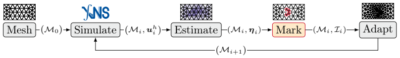
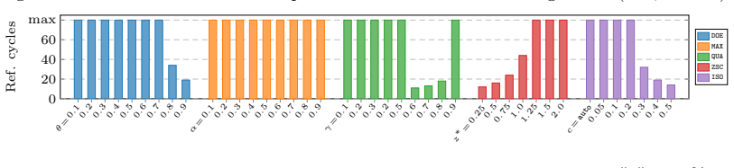
The study benchmarks marking strategies for adaptive mesh refinement driven by the Kelly residual estimator on steady mechanics problems. It concludes that quantile and z-score markings are the most robust, Dörfler marking is effective when using large bulk parameters, maximum marking is sensitive to irregular fields, and Isolation Forest can match top performers only with generous contamination settings but risks failure under aggressive parameters.
What carries the argument
Marking strategies applied to elements selected by the residual-based Kelly error estimator, including maximum, Dörfler, quantile, z-score, and Isolation Forest methods.
If this is right
- Quantile and z-score markings maintain consistent performance across different problem types and field characteristics.
- Dörfler marking achieves good results when the bulk parameter is chosen sufficiently large.
- Maximum marking can lead to overly sensitive or irregular refinement patterns in solutions with varying smoothness.
- Isolation Forest requires a sufficiently high contamination parameter to match classical methods but becomes unreliable if set too aggressively.
- Selecting robust marking strategies can help reduce overall computational costs in adaptive finite element workflows.
Where Pith is reading between the lines
- The preference for quantile and z-score methods might apply to time-dependent or multiphysics simulations if the error estimator behaves similarly.
- Alternative error estimators could alter which marking strategy ranks highest, suggesting the need for problem-specific validation.
- In very large-scale computations, the efficiency gains from robust marking could translate to significant savings in time and resources.
- Hybrid strategies that combine quantile marking with elements of Isolation Forest might offer further improvements.
Load-bearing premise
The steady solid and fluid mechanics test problems paired with the residual-based Kelly error estimator are representative of broader engineering applications.
What would settle it
Repeating the benchmark study using transient problems or a different error estimator such as the Zienkiewicz-Zhu method and finding that the robustness order of the marking strategies changes would falsify the generalizability of these results.
Figures


read the original abstract
Adaptive mesh refinement (AMR) is indispensable for efficient finite element analyses. However, its performance depends not only on the refinement itself but also on strategy to mark elements for refinement and the way it is tuned. This work compares classical marking methods (maximum, D\"orfler bulk-chasing, quantile) with non-classical, statistically based approaches (z-score, Isolation Forest), all driven by the residual-based Kelly error estimator and tested on steady solid and fluid mechanics problems. The study finds quantile and z-score markings to be the most robust, D\"orfler effective for large bulk parameters, and maximum marking sensitive to irregular fields. Isolation Forest can rival top classical methods with a generous contamination level but may fail under aggressive settings. These results offer practical guidance for selecting marking strategies that balance refinement aggressiveness and computational cost in adaptive FEM workflows.
Editorial analysis
A structured set of objections, weighed in public.
Referee Report
Summary. The manuscript presents a benchmark study comparing classical marking strategies (maximum, Dörfler bulk-chasing, quantile) with statistical approaches (z-score, Isolation Forest) for adaptive mesh refinement in finite element methods. All strategies are driven by the residual-based Kelly error estimator and tested on steady solid and fluid mechanics problems. The central claim is that quantile and z-score markings are the most robust, Dörfler is effective for large bulk parameters, maximum marking is sensitive to irregular fields, and Isolation Forest can rival the top classical methods when the contamination level is set generously but may fail under aggressive settings. These findings are positioned as practical guidance for balancing refinement aggressiveness and computational cost in AMR workflows.
Significance. If the reported performance orderings hold, the work supplies useful empirical data on marking strategy selection for AMR, extending prior comparisons by including non-classical statistical methods. The efficiency-focused framing and use of a standard residual estimator are strengths for practitioners in solid and fluid mechanics FEM. However, the significance is constrained by the narrow problem class and the qualitative presentation of robustness rankings, limiting immediate applicability to broader engineering workloads.
major comments (2)
- [Abstract and Results] The robustness rankings (quantile/z-score most robust; maximum sensitive to irregular fields) are load-bearing for the practical guidance claim yet rest on qualitative summaries of performance across the chosen test problems. No quantitative metrics such as error-vs-DOF curves with error bars, wall-clock timings, or mesh statistics are referenced in the abstract or results, and no statistical tests of variability are reported, making it impossible to assess the magnitude or significance of differences between strategies.
- [Discussion and Conclusions] The claim that the observed orderings provide general practical guidance assumes the selected steady solid- and fluid-mechanics problems together with the Kelly estimator adequately sample real engineering variability. No sensitivity study to problem selection, geometry, singularities, nonlinearity, or alternative error indicators is presented; an atypical test suite could invert the rankings without contradicting the reported data.
minor comments (2)
- [Methods] The methods section should explicitly tabulate the exact parameter values used for each strategy (e.g., bulk parameter range for Dörfler, contamination levels for Isolation Forest, z-score threshold) so that the experiments are fully reproducible.
- [Figures] Figure captions and legends would benefit from clearer indication of which curves correspond to which marking strategy and parameter setting, especially when multiple contamination levels are shown for Isolation Forest.
Simulated Author's Rebuttal
We thank the referee for the constructive feedback on our benchmark study of marking strategies for adaptive mesh refinement. We address each major comment below, proposing targeted revisions to improve clarity and balance while preserving the manuscript's focus and scope.
read point-by-point responses
-
Referee: [Abstract and Results] The robustness rankings (quantile/z-score most robust; maximum sensitive to irregular fields) are load-bearing for the practical guidance claim yet rest on qualitative summaries of performance across the chosen test problems. No quantitative metrics such as error-vs-DOF curves with error bars, wall-clock timings, or mesh statistics are referenced in the abstract or results, and no statistical tests of variability are reported, making it impossible to assess the magnitude or significance of differences between strategies.
Authors: We acknowledge that the abstract and results summaries are primarily descriptive. The manuscript does contain error-versus-DOF curves, mesh statistics, and comparative performance data in the results section and figures, but these are presented visually without explicit numerical call-outs or variability measures in the text. To strengthen the presentation, we will revise the abstract to reference key quantitative trends (such as typical DOF counts at target error levels) and enhance the results section with additional quantitative summaries, error bars on relevant plots where feasible, and notes on the magnitude of observed differences. Wall-clock timings for the marking step itself can be added as supplementary data, though the primary efficiency metric remains error reduction per degree of freedom. Full statistical hypothesis testing across all problems would require additional analysis but can be noted as a limitation. revision: partial
-
Referee: [Discussion and Conclusions] The claim that the observed orderings provide general practical guidance assumes the selected steady solid- and fluid-mechanics problems together with the Kelly estimator adequately sample real engineering variability. No sensitivity study to problem selection, geometry, singularities, nonlinearity, or alternative error indicators is presented; an atypical test suite could invert the rankings without contradicting the reported data.
Authors: We agree that the reported orderings are tied to the specific steady problems and residual-based Kelly estimator used. The manuscript frames the work as a focused benchmark study rather than a universal claim, but we will strengthen the discussion and conclusions by explicitly qualifying the practical guidance as applicable to the tested class of problems. A dedicated limitations section will be added to note that rankings could vary with different geometries, singularities, nonlinearities, or error indicators, and to recommend case-specific validation. A comprehensive sensitivity study across all such variations lies beyond the scope of this efficiency-focused comparison of marking strategies. revision: partial
Circularity Check
No significant circularity in empirical benchmark study
full rationale
The paper conducts a direct empirical comparison of marking strategies (maximum, Dörfler, quantile, z-score, Isolation Forest) for AMR, all driven by the residual-based Kelly estimator on a suite of steady solid- and fluid-mechanics test problems. No mathematical derivations, parameter fittings, or predictive claims are made that could reduce to inputs by construction. Results consist solely of observed performance metrics (robustness, efficiency) from numerical experiments. Any self-citations are incidental and non-load-bearing for the reported rankings, which rest on the external test problems rather than internal definitions or prior author results. This is a standard benchmark paper whose findings are falsifiable by rerunning the experiments on different problems or estimators.
Axiom & Free-Parameter Ledger
Reference graph
Works this paper leans on
-
[1]
A posteriori error estimation in finite element analysis.Computer methods in applied mechanics and engineering, 142(1-2):1–88, 1997
Mark Ainsworth and J Tinsley Oden. A posteriori error estimation in finite element analysis.Computer methods in applied mechanics and engineering, 142(1-2):1–88, 1997
1997
-
[2]
OUP Oxford, 2013
Rüdiger Verfürth.A posteriori error estimation techniques for finite element methods. OUP Oxford, 2013
2013
-
[3]
A convergent adaptive algorithm for poisson’s equation.SIAM Journal on Numerical Analysis, 33(3):1106–1124, 1996
Willy Dörfler. A convergent adaptive algorithm for poisson’s equation.SIAM Journal on Numerical Analysis, 33(3):1106–1124, 1996
1996
-
[4]
Convergence of adaptive finite element methods.SIAM review, 44(4):631–658, 2002
Pedro Morin, Ricardo H Nochetto, and Kunibert G Siebert. Convergence of adaptive finite element methods.SIAM review, 44(4):631–658, 2002
2002
-
[5]
A posteriori error analysis and adaptive processes in the finite element method: Part i—error analysis
Donald W Kelly, JP De SR Gago, Olgierd C Zienkiewicz, and Ivo Babuska. A posteriori error analysis and adaptive processes in the finite element method: Part i—error analysis. International journal for numerical methods in engineering, 19(11):1593–1619, 1983
1983
-
[6]
JP De SR Gago, Donald W Kelly, Olgierd C Zienkiewicz, and I Babuska. A posteriori error analysis and adaptive processes in the finite element method: Part ii—adaptive mesh refinement.International journal for numerical methods in engineering, 19(11):1621–1656, 1983
1983
-
[7]
High accuracy mantle convec- tion simulation through modern numerical methods.Geophysical Journal International, 191(1):12–29, 2012
Martin Kronbichler, Timo Heister, and Wolfgang Bangerth. High accuracy mantle convec- tion simulation through modern numerical methods.Geophysical Journal International, 191(1):12–29, 2012
2012
-
[8]
Wolfgang Bangerth, Ralf Hartmann, and Guido Kanschat. deal. ii—a general-purpose object-oriented finite element library.ACM Transactions on Mathematical Software (TOMS), 33(4):24–es, 2007
2007
-
[9]
Optimality of a standard adaptive finite element method.Foundations of Computational Mathematics, 7(2):245–269, 2007
Rob Stevenson. Optimality of a standard adaptive finite element method.Foundations of Computational Mathematics, 7(2):245–269, 2007
2007
-
[10]
Quasi-optimal convergence rate for an adaptive finite element method.SIAM Journal on Numerical Analysis, 46(5):2524–2550, 2008
J Manuel Cascon, Christian Kreuzer, Ricardo H Nochetto, and Kunibert G Siebert. Quasi-optimal convergence rate for an adaptive finite element method.SIAM Journal on Numerical Analysis, 46(5):2524–2550, 2008
2008
-
[11]
Adaptive finite element methods with convergence rates.Numerische Mathematik, 97(2):219–268, 2004
Peter Binev, Wolfgang Dahmen, and Ron DeVore. Adaptive finite element methods with convergence rates.Numerische Mathematik, 97(2):219–268, 2004
2004
-
[12]
Malú Grave and Alvaro L. G. A. Coutinho. Adaptive mesh refinement and coarsening for diffusion–reaction epidemiological models.Computational Mechanics, 67(4):1177–1199, 2021
2021
-
[13]
Adaptive refinement in advection–diffusion problems by anomaly detection: A numerical study.Algorithms, 14(11), 2021
Antonella Falini and Maria Lucia Sampoli. Adaptive refinement in advection–diffusion problems by anomaly detection: A numerical study.Algorithms, 14(11), 2021
2021
-
[14]
Learning robust marking policies for adaptive mesh refinement.SIAM Journal on Scientific Computing, 46:A264–A289, 2024
Andrew Gillette, Brendan Keith, and Socratis Petrides. Learning robust marking policies for adaptive mesh refinement.SIAM Journal on Scientific Computing, 46:A264–A289, 2024. 14
2024
-
[15]
Recurrent neural networks as optimal mesh refinement strategies.Computers and Mathematics with Applications, 97:61–76, 2021
Jan Bohn and Michael Feischl. Recurrent neural networks as optimal mesh refinement strategies.Computers and Mathematics with Applications, 97:61–76, 2021
2021
-
[16]
Isolation forest
Fei Tony Liu, Kai Ming Ting, and Zhi-Hua Zhou. Isolation forest. In2008 eighth ieee international conference on data mining, pages 413–422. IEEE, 2008
2008
-
[17]
Springer Science & Business Media, 2003
Wolfgang Bangerth and Rolf Rannacher.Adaptive finite element methods for differential equations. Springer Science & Business Media, 2003
2003
-
[18]
Multi-level hp-adaptivity: high-order mesh adaptivity without the difficulties of constrain- ing hanging nodes.Computational Mechanics, 55(3):499–517, 2015
Nils Zander, Tino Bog, Stefan Kollmannsberger, Dominik Schillinger, and Ernst Rank. Multi-level hp-adaptivity: high-order mesh adaptivity without the difficulties of constrain- ing hanging nodes.Computational Mechanics, 55(3):499–517, 2015
2015
-
[19]
Gmsh: A 3-d finite element mesh gen- erator with built-in pre-and post-processing facilities.International journal for numerical methods in engineering, 79(11):1309–1331, 2009
Christophe Geuzaine and Jean-François Remacle. Gmsh: A 3-d finite element mesh gen- erator with built-in pre-and post-processing facilities.International journal for numerical methods in engineering, 79(11):1309–1331, 2009
2009
-
[20]
A posteriori error estimation and adaptive mesh-refinement techniques
Rüdiger Verfürth. A posteriori error estimation and adaptive mesh-refinement techniques. Journal of Computational and Applied Mathematics, 50(1):67–83, 1994
1994
-
[21]
Nochetto, Kunibert G
Ricardo H. Nochetto, Kunibert G. Siebert, and Andreas Veeser. Theory of adaptive finite element methods: An introduction. InMultiscale, Nonlinear and Adaptive Approximation, pages 409–542. Springer Berlin Heidelberg, 2009
2009
-
[22]
A basic convergence result for conforming adaptive finite elements.Mathematical Models and Methods in Applied Sciences, 18(05):707–737, 2008
Pedro Morin, Kunibert G Siebert, and Andreas Veeser. A basic convergence result for conforming adaptive finite elements.Mathematical Models and Methods in Applied Sciences, 18(05):707–737, 2008
2008
-
[23]
Adaptive mesh refinement strategies in isogeometric analysis— a computational comparison.Computer Methods in Applied Mechanics and Engineering, 316:424–448, 2017
Paul Hennig, Markus Kästner, Philipp Morgenstern, and Daniel Peterseim. Adaptive mesh refinement strategies in isogeometric analysis— a computational comparison.Computer Methods in Applied Mechanics and Engineering, 316:424–448, 2017
2017
-
[24]
Outlier detection using isolation forest and local outlier factor
Zhangyu Cheng, Chengming Zou, and Jianwei Dong. Outlier detection using isolation forest and local outlier factor. InProceedings of the Conference on Research in Adaptive and Convergent Systems, pages 161–168. Association for Computing Machinery, 2019
2019
-
[25]
Scikit-learn: Machine learning in python.the Journal of machine Learning research, 12:2825–2830, 2011
Fabian Pedregosa, Gaël Varoquaux, Alexandre Gramfort, Vincent Michel, Bertrand Thirion, Olivier Grisel, Mathieu Blondel, Peter Prettenhofer, Ron Weiss, Vincent Dubourg, et al. Scikit-learn: Machine learning in python.the Journal of machine Learning research, 12:2825–2830, 2011
2011
-
[26]
SIAM, 2002
Philippe G Ciarlet.The finite element method for elliptic problems. SIAM, 2002
2002
-
[27]
SIAM, 2011
Pierre Grisvard.Elliptic problems in nonsmooth domains. SIAM, 2011
2011
-
[28]
John Wiley & Sons, 2003
Jean Donea and Antonio Huerta.Finite element methods for flow problems. John Wiley & Sons, 2003
2003
-
[29]
Estimation and control of error based on p convergence.Accuracy estimates and adaptive refinements in finite element computations, 1:61–70, 1986
Barna A Szabó. Estimation and control of error based on p convergence.Accuracy estimates and adaptive refinements in finite element computations, 1:61–70, 1986
1986
-
[30]
Academic Press, 2009
Martin H Sadd.Elasticity: theory, applications, and numerics. Academic Press, 2009
2009
-
[31]
John Wiley & Sons, 2009
J Austin Cottrell, Thomas JR Hughes, and Yuri Bazilevs.Isogeometric analysis: toward integration of CAD and FEA. John Wiley & Sons, 2009
2009
-
[32]
Dominik Schillinger and Martin Ruess. The finite cell method: a review in the context of higher-order structural analysis of cad and image-based geometric models.Archives of Computational Methods in Engineering, 22(3):391–455, 2015. 15
2015
-
[33]
High-re solutions for incompressible flow using the navier-stokes equations and a multigrid method.Journal of computational physics, 48(3):387–411, 1982
UKNG Ghia, Kirti N Ghia, and CT Shin. High-re solutions for incompressible flow using the navier-stokes equations and a multigrid method.Journal of computational physics, 48(3):387–411, 1982
1982
-
[34]
Bench- mark computations of laminar flow around a cylinder
Michael Schäfer, Stefan Turek, Franz Durst, Egon Krause, and Rolf Rannacher. Bench- mark computations of laminar flow around a cylinder. InFlow simulation with high- performance computers II: DFG priority research programme results 1993–1995, pages 547–566. Springer, 1996. 16
1993
discussion (0)
Sign in with ORCID, Apple, or X to comment. Anyone can read and Pith papers without signing in.