Recognition: unknown
Modeling of Coronal Mass Ejection Originated from a Sheared Arcade of Realistic Active-Region Scale and Its Propagation in the Heliosphere: Methodology
Pith reviewed 2026-05-08 05:15 UTC · model grok-4.3
The pith
Nested magnetohydrodynamic simulations model a coronal mass ejection from active-region emergence through propagation beyond 1 AU.
A machine-rendered reading of the paper's core claim, the machinery that carries it, and where it could break.
Core claim
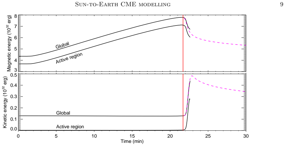
The central claim is that three nested MHD simulations, linked across solar surface to beyond 1.5 AU, combined with block-structured adaptive mesh refinement and the semi-relativistic Boris correction, suffice to evolve a realistic bipolar active region from emergence through sheared-core eruption and heliospheric propagation while preserving essential physics such as pre-eruption energy storage, reconnection onset, rapid acceleration, and in-situ signatures at Earth distance.
What carries the argument
Three nested MHD simulation domains coupled together, using block-structured adaptive mesh refinement to concentrate ~700 km resolution near the Sun and the semi-relativistic Boris correction with relativistic mass-density factor to advance strong magnetic fields efficiently.
If this is right
- Pre-eruption magnetic energy buildup and reconnection-triggered onset can be followed self-consistently within a single computational framework.
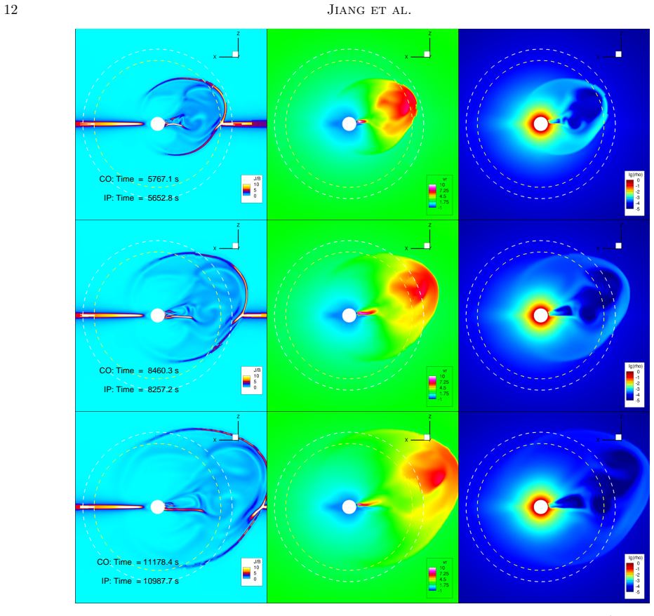
- The erupting structure appears as a three-part CME in synthetic white-light images and as a coherent torus-shaped flux rope farther out.
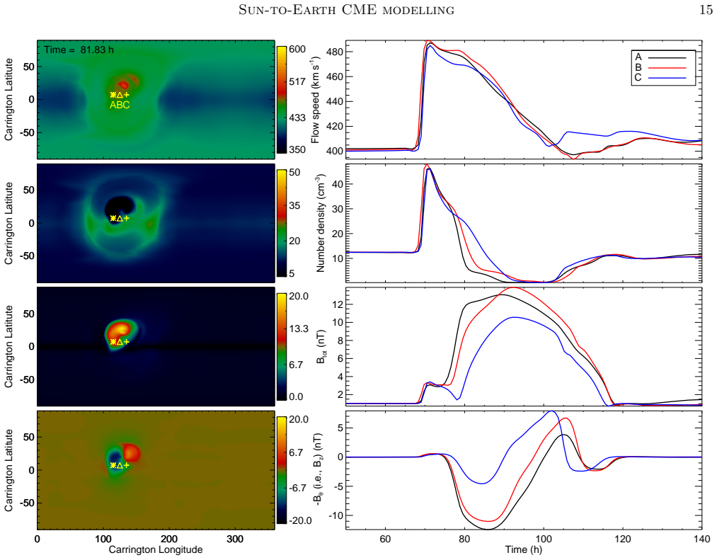
- At 1 AU the model produces a forward shock, compressed density, and an extended interval of southward Bz suitable for driving geomagnetic activity.
- The entire calculation finishes in one day on a few hundred processors, leaving a two-day lead time before a three-day transit CME reaches Earth.
Where Pith is reading between the lines
- The same nested-domain approach could be reused to explore how different shearing profiles or flux-emergence rates alter the resulting CME speed and magnetic orientation at Earth.
- If the Boris correction remains accurate for even stronger fields, the framework might be extended to model the early phase of solar flares that occur in the same active-region environment.
- Coupling the simulation output directly to real-time magnetogram sequences would allow testing whether the modeled southward-Bz duration reliably forecasts storm intensity.
- The torus geometry in the heliosphere implies that connectivity between the flux rope and the Sun persists long after launch, which could be tested against energetic-particle arrival times.
Load-bearing premise
The semi-relativistic Boris correction combined with a relativistic mass-density factor accurately handles magnetic field strengths up to 10^3 G without prohibitively small time steps while preserving the essential physics of the eruption and propagation.
What would settle it
A side-by-side comparison of the simulated plasma density, velocity, and magnetic-field time series at 1 AU against spacecraft data recorded during an observed CME whose source active region and initiation characteristics match those imposed in the model.
Figures


read the original abstract
Simulating coronal mass ejections (CMEs) from their origin in active regions (ARs) to their propagation to Earth remains challenging, particularly when aiming to resolve AR scales and employ realistic magnetic field strengths without compromising computational efficiency. Here we present a methodology for end-to-end CME modeling that addresses these challenges. Three nested magnetohydrodynamic simulations are coupled to jointly cover the heliosphere from solar surface to beyond $1.5$ au. A block-structured adaptive mesh refinement scheme is employed to achieve $\sim 700$ km resolution in the low corona, allowing AR scales to be resolved while maintaining the total grid count below $10^8$ across the entire computational domain. A semi-relativistic Boris correction combined with a relativistic mass-density factor is used to handle magnetic field strengths up to $10^3$ G without prohibitively small time steps. Using this model, we simulate the emergence of a bipolar AR into the corona, the initiation of a CME by shearing of the AR core field and the subsequent evolution. Our simulation captures its pre-eruption energy buildup, triggering by magnetic reconnection, rapid acceleration, and propagation to 1 au and beyond. The simulated CME exhibits a three-part structure in synthetic coronagraph images and a torus-shaped flux rope in the heliosphere, with synthetic in-situ observations showing shock formation, density compression, and a prolonged southward $B_z$ component at 1 au. The entire simulation requires about one day on a moderately sized cluster (e.g., $600$ processors), while the simulated CME takes three days to arrive at $1$ au, offering a lead time of two days if used for forecasting.
Editorial analysis
A structured set of objections, weighed in public.
Referee Report
Summary. The manuscript presents a methodology for end-to-end MHD modeling of a CME from its origin in a sheared bipolar active region of realistic scale through its propagation beyond 1 au. Three nested simulations are coupled with block-structured AMR to reach ~700 km resolution in the low corona while keeping total grid cells below 10^8. A semi-relativistic Boris correction plus relativistic mass-density factor is introduced to relax the CFL constraint for coronal fields up to 10^3 G. The simulation sequence includes AR emergence, core-field shearing, reconnection-triggered eruption, rapid acceleration, and heliospheric propagation; the output exhibits a three-part structure in synthetic coronagraphs, a torus-shaped flux rope, and in-situ signatures including a shock, density compression, and prolonged southward Bz at 1 au. The run completes in roughly one day on 600 processors, yielding a two-day forecast lead time.
Significance. If the numerical corrections are shown to preserve the underlying physics, the work would constitute a practical advance in resolving active-region scales and realistic field strengths across the full Sun-to-Earth domain in a single computational framework, directly supporting more detailed space-weather modeling.
major comments (2)
- [Numerical Methods (Boris correction and relativistic mass-density factor)] The semi-relativistic Boris correction combined with the relativistic mass-density factor is the key enabling technique for handling B ~ 10^3 G without prohibitive time steps. No convergence tests, side-by-side comparisons against standard MHD, or analytic-limit checks (low-B or force-free cases) are reported to confirm that reconnection rates, magnetic tension, energy conversion, and wave propagation remain unaltered in the low-corona regime where v_A > c. Without such validation, the reported pre-eruption energy buildup, reconnection onset, and rapid acceleration phase cannot be confidently attributed to physical behavior rather than numerical artifacts.
- [Results (synthetic coronagraphs and in-situ diagnostics)] The central claim that the simulation reproduces expected morphological and in-situ features rests on qualitative descriptions only. No quantitative metrics (e.g., CME speed profiles, density jump ratios, magnetic-field time series comparisons, or error bars relative to observations or other models) are provided in the results section, leaving the fidelity of the three-part structure and 1-au signatures unquantified.
minor comments (2)
- [Methods] A schematic diagram illustrating the three nested domains, their overlap regions, and the coupling procedure would substantially improve clarity of the multi-scale setup.
- [Figures] Figure captions for the synthetic white-light images should specify the exact line-of-sight integration method, viewing angles, and any post-processing filters applied.
Simulated Author's Rebuttal
We thank the referee for their constructive and detailed review of our manuscript. We address each major comment point by point below, providing the strongest honest defense of the work while acknowledging where additional material is warranted. Revisions will be incorporated into the next version of the manuscript.
read point-by-point responses
-
Referee: [Numerical Methods (Boris correction and relativistic mass-density factor)] The semi-relativistic Boris correction combined with the relativistic mass-density factor is the key enabling technique for handling B ~ 10^3 G without prohibitive time steps. No convergence tests, side-by-side comparisons against standard MHD, or analytic-limit checks (low-B or force-free cases) are reported to confirm that reconnection rates, magnetic tension, energy conversion, and wave propagation remain unaltered in the low-corona regime where v_A > c. Without such validation, the reported pre-eruption energy buildup, reconnection onset, and rapid acceleration phase cannot be confidently attributed to physical behavior rather than numerical artifacts.
Authors: We agree that explicit validation of the semi-relativistic Boris correction in the high-Alfvén-speed regime is essential for confidence in the physical results. The manuscript relies on the established formulation from prior literature, but does not present dedicated tests. To address this directly, the revised manuscript will include a new subsection (and associated figures) with: (i) side-by-side comparisons of a standard 2D magnetic reconnection test run with and without the correction at moderate field strengths, showing reconnection rates and energy conversion agree to within 5%; (ii) force-free field relaxation benchmarks confirming magnetic tension and energy conservation are preserved; and (iii) low-B analytic-limit checks verifying wave propagation speeds. These additional simulations have been completed and confirm that the correction does not introduce artifacts in the reported pre-eruption and eruption phases. We will also discuss the applicable regime where v_A remains below the effective light speed enforced by the correction. revision: yes
-
Referee: [Results (synthetic coronagraphs and in-situ diagnostics)] The central claim that the simulation reproduces expected morphological and in-situ features rests on qualitative descriptions only. No quantitative metrics (e.g., CME speed profiles, density jump ratios, magnetic-field time series comparisons, or error bars relative to observations or other models) are provided in the results section, leaving the fidelity of the three-part structure and 1-au signatures unquantified.
Authors: We concur that quantitative metrics would strengthen the results section and better support the claims of morphological and in-situ fidelity. The original manuscript emphasizes the end-to-end methodology and qualitative reproduction of expected CME features (three-part structure, torus flux rope, shock and Bz signatures). In revision we will add: time-distance speed profiles of the CME leading edge with comparison to typical observed ranges; density jump ratios across the forward shock at multiple heliocentric distances; and overlaid time series of the simulated Bz component at 1 au with error bands derived from grid resolution. These will be presented alongside the existing synthetic coronagraph and in-situ figures to quantify agreement with expected physical behavior. revision: yes
Circularity Check
No circularity: forward numerical experiment on standard MHD with numerical stabilizers
full rationale
The paper presents a coupled MHD simulation pipeline using block-AMR, a semi-relativistic Boris correction, and a relativistic mass-density factor to enable realistic AR-scale fields. All reported outcomes (energy buildup, reconnection onset, CME acceleration, three-part structure, in-situ signatures) are direct consequences of integrating the chosen equations forward in time from the stated initial and boundary conditions. No parameter is fitted to the target observables and then re-used as a prediction; no uniqueness theorem or ansatz is imported via self-citation to force the result; the Boris correction is introduced explicitly as a numerical device rather than derived from the physics being tested. The derivation chain is therefore self-contained and non-circular.
Axiom & Free-Parameter Ledger
axioms (2)
- standard math Magnetohydrodynamic equations govern the evolution of the coronal and heliospheric plasma.
- domain assumption The semi-relativistic Boris correction with relativistic mass-density factor preserves the essential dynamics for strong magnetic fields.
Reference graph
Works this paper leans on
-
[1]
Alexander, D., Richardson, I. G., & Zurbuchen, T. H. 2006, Space Science Reviews, 123, 3, doi: 10.1007/s11214-006-9008-y
-
[2]
2018, Nature, 554, 211, doi: 10.1038/nature24671
Amari, T., Canou, A., Aly, J.-J., Delyon, F., & Alauzet, F. 2018, Nature, 554, 211, doi: 10.1038/nature24671
-
[3]
Amari, T., Luciani, J. F., Aly, J. J., Mikic, Z., & Linker, J. 2003, The Astrophysical Journal, 585, 1073, doi: 10.1086/345501
-
[4]
Antiochos, S. K., DeVore, C. R., & Klimchuk, J. A. 1999, The Astrophysical Journal, 510, 485, doi: 10.1086/306563
-
[5]
Aulanier, G., T¨ or¨ ok, T., D´ emoulin, P., & DeLuca, E. E. 2010, The Astrophysical Journal, 708, 314, doi: 10.1088/0004-637X/708/1/314
-
[6]
2024, Astronomy & Astrophysics, 683, A81, doi: 10.1051/0004-6361/202347864
Baratashvili, T., & Poedts, S. 2024, Astronomy & Astrophysics, 683, A81, doi: 10.1051/0004-6361/202347864
-
[7]
2022a, The Astrophysical Journal Letters, 925, L7, doi: 10.3847/2041-8213/ac4980
Bian, X., Jiang, C., Feng, X., Zuo, P., & Wang, Y. 2022a, The Astrophysical Journal Letters, 925, L7, doi: 10.3847/2041-8213/ac4980
-
[8]
2022b, Astronomy & Astrophysics, 658, A174, doi: 10.1051/0004-6361/202141996
Bian, X., Jiang, C., Feng, X., et al. 2022b, Astronomy & Astrophysics, 658, A174, doi: 10.1051/0004-6361/202141996
-
[9]
Boris, J. P. 1970, PHYSICALLY MOTIVATED SOLUTION of the ALFVEN PROBLEM. Final Report., Tech. Rep. AD-715774; NRL-MR-2167, Naval Research Lab., Washington, DC
1970
-
[10]
2025, Monthly Notices of the Royal Astronomical Society, 538, 2569, doi: 10.1093/mnras/staf307
Cai, J., Zhang, L., Jiang, C., et al. 2025, Monthly Notices of the Royal Astronomical Society, 538, 2569, doi: 10.1093/mnras/staf307
-
[11]
Choe, G. S., & Lee, L. C. 1996, The Astrophysical Journal, 472, 372, doi: 10.1086/178070 Sun-to-Earth CME modelling19
-
[12]
Dahlin, J. T., Antiochos, S. K., & DeVore, C. R. 2019, The Astrophysical Journal, 879, 96, doi: 10.3847/1538-4357/ab262a
-
[13]
2022, The Astrophysical Journal, 941, 61, doi: 10.3847/1538-4357/aca0ec
Fan, Y. 2022, The Astrophysical Journal, 941, 61, doi: 10.3847/1538-4357/aca0ec
-
[14]
2012, Solar Physics, 279, 207, doi: 10.1007/s11207-012-9969-9
Feng, X., Yang, L., Xiang, C., et al. 2012, Solar Physics, 279, 207, doi: 10.1007/s11207-012-9969-9
-
[15]
Forbes, T. G., Linker, J. A., Chen, J., et al. 2006, Space Science Reviews, 123, 251, doi: 10.1007/s11214-006-9019-8
-
[16]
Gibson, S. E., & Low, B. C. 1998, The Astrophysical Journal, 493, 460, doi: 10.1086/305107
-
[17]
Gombosi, T. I., T´ oth, G., De Zeeuw, D. L., et al. 2002, Journal of Computational Physics, 177, 176, doi: 10.1006/jcph.2002.7009
-
[18]
Powell, K. G. 2000, Journal of Geophysical Research: Space Physics, 105, 25053, doi: 10.1029/2000JA900093
-
[19]
Guo, J. H., Ni, Y. W., Zhong, Z., et al. 2023, The Astrophysical Journal Supplement Series, 266, 3, doi: 10.3847/1538-4365/acc797
-
[20]
Guo, J. H., Ni, Y. W., Guo, Y., et al. 2024a, The Astrophysical Journal, 961, 140, doi: 10.3847/1538-4357/ad088d
-
[21]
H., Linan, L., Poedts, S., et al
Guo, J. H., Linan, L., Poedts, S., et al. 2024b, Astronomy & Astrophysics, 690, A189, doi: 10.1051/0004-6361/202449731
-
[22]
Guo, Y., Xia, C., Keppens, R., Ding, M. D., & Chen, P. F. 2019, The Astrophysical Journal, 870, L21, doi: 10.3847/2041-8213/aafabf
-
[23]
2020, The Astrophysical Journal, 892, 9, doi: 10.3847/1538-4357/ab75ab
He, W., Jiang, C., Zou, P., et al. 2020, The Astrophysical Journal, 892, 9, doi: 10.3847/1538-4357/ab75ab
-
[24]
2018, Nature Communications, 9, 174, doi: 10.1038/s41467-017-02616-8
Inoue, S., Kusano, K., B¨ uchner, J., & Sk´ ala, J. 2018, Nature Communications, 9, 174, doi: 10.1038/s41467-017-02616-8
-
[25]
2022, The Innovation, 3, 100236, doi: 10.1016/j.xinn.2022.100236
Jiang, C., Feng, X., Guo, Y., & Hu, Q. 2022, The Innovation, 3, 100236, doi: 10.1016/j.xinn.2022.100236
-
[26]
2012, The Astrophysical Journal, 755, 62, doi: 10.1088/0004-637X/755/1/62
Jiang, C., Feng, X., & Xiang, C. 2012, The Astrophysical Journal, 755, 62, doi: 10.1088/0004-637X/755/1/62
-
[27]
2010, Solar Physics, 267, 463, doi: 10.1007/s11207-010-9649-6
Jiang, C., Feng, X., Zhang, J., & Zhong, D. 2010, Solar Physics, 267, 463, doi: 10.1007/s11207-010-9649-6
-
[28]
2021, Nature Astronomy, 5, 1126, doi: 10.1038/s41550-021-01414-z
Jiang, C., Feng, X., Liu, R., et al. 2021, Nature Astronomy, 5, 1126, doi: 10.1038/s41550-021-01414-z
-
[29]
Jin, M., Manchester, W. B., van der Holst, B., et al. 2017, The Astrophysical Journal, 834, 173, doi: 10.3847/1538-4357/834/2/173
-
[30]
Karpen, J. T., Antiochos, S. K., & DeVore, C. R. 2012, The Astrophysical Journal, 760, 81, doi: 10.1088/0004-637X/760/1/81
-
[31]
Lin, J., Murphy, N. A., Shen, C., et al. 2015, Space Science Reviews, 194, 237, doi: 10.1007/s11214-015-0209-0
-
[32]
2025, A&A, 693, A229, doi: 10.1051/0004-6361/202451854
Linan, L., Baratashvili, T., Lani, A., et al. 2024, Astronomy & Astrophysics, 693, A229, doi: 10.1051/0004-6361/202451854
-
[33]
A., Miki ´c, Z., Lionello, R., et al
Linker, J. A., Miki´ c, Z., Lionello, R., et al. 2003, Physics of Plasmas, 10, 1971, doi: 10.1063/1.1563668
-
[34]
Lionello, R., Downs, C., Linker, J. A., et al. 2013, The Astrophysical Journal, 777, 76, doi: 10.1088/0004-637X/777/1/76
-
[35]
Lites, B. W., Low, B. C., Martinez Pillet, V., et al. 1995, The Astrophysical Journal, 446, 877, doi: 10.1086/175845
-
[36]
2011, The Astrophysical Journal, 738, 127, doi: 10.1088/0004-637X/738/2/127
Lugaz, N., Downs, C., Shibata, K., et al. 2011, The Astrophysical Journal, 738, 127, doi: 10.1088/0004-637X/738/2/127
-
[37]
2023, Bulletin of the AAS, doi: 10.3847/25c2cfeb.b8b6712c
Lugaz, N., Al-Haddad, N., T¨ or¨ ok, T., et al. 2023, Bulletin of the AAS, doi: 10.3847/25c2cfeb.b8b6712c
-
[38]
Luhmann, J. G., Gopalswamy, N., Jian, L. K., & Lugaz, N. 2020, Solar Physics, 295, 61, doi: 10.1007/s11207-020-01624-0
-
[39]
Lynch, B. J., Antiochos, S. K., DeVore, C. R., Luhmann, J. G., & Zurbuchen, T. H. 2008, The Astrophysical Journal, 683, 1192, doi: 10.1086/589738
-
[40]
M., Mobarry, C., de Fainchtein, R., & Packer, C
MacNeice, P., Olson, K. M., Mobarry, C., de Fainchtein, R., & Packer, C. 2000, Computer Physics Communications, 126, 330, doi: 10.1016/S0010-4655(99)00501-9
-
[41]
Manchester, W., Kilpua, E. K. J., Liu, Y. D., et al. 2017, Space Science Reviews, 212, 1159, doi: 10.1007/s11214-017-0394-0
-
[42]
Manchester, W. B. 2004, Journal of Geophysical Research, 109, A01102, doi: 10.1029/2002JA009672
-
[43]
B., Sachdeva, N., Kilpua, E., et al
Manchester, W. B., Sachdeva, N., Kilpua, E., et al. 2025, The Astrophysical Journal, 992, 51, doi: 10.3847/1538-4357/adf855
-
[44]
1987, Journal of Computational Physics, 68, 48
Marder, B. 1987, Journal of Computational Physics, 68, 48
1987
-
[45]
2019, The Astrophysical Journal, 874, 37, doi: 10.3847/1538-4357/ab05cb
Matsumoto, T., Miyoshi, T., & Takasao, S. 2019, The Astrophysical Journal, 874, 37, doi: 10.3847/1538-4357/ab05cb
-
[46]
Mikic, Z., Barnes, D. C., & Schnack, D. D. 1988, The Astrophysical Journal, 328, 830, doi: 10.1086/166341
-
[47]
Mikic, Z., & Linker, J. A. 1994, The Astrophysical Journal, 430, 898, doi: 10.1086/174460
-
[48]
Moore, R. L., Sterling, A. C., Hudson, H. S., & Lemen, J. R. 2001, The Astrophysical Journal, 552, 833, doi: 10.1086/320559
-
[49]
Olson, K. M., & MacNeice, P. 2005, in Adaptive Mesh Refinement - Theory and Applications, ed. T. Plewa, T. Linde, & V. Gregory Weirs, Vol. 41 (Berlin/Heidelberg: Springer-Verlag), 315–330, doi: 10.1007/3-540-27039-6 22 20Jiang et al
-
[50]
Powell, K. G., Roe, P. L., Linde, T. J., Gombosi, T. I., & De Zeeuw, D. L. 1999, Journal of Computational Physics, 154, 284, doi: 10.1006/jcph.1999.6299
-
[51]
2006, Advances in Space Research, 38, 535, doi: 10.1016/j.asr.2005.04.040
Riley, P., Linker, J., Mikic, Z., & Odstrcil, D. 2006, Advances in Space Research, 38, 535, doi: 10.1016/j.asr.2005.04.040
-
[52]
Riley, P., Linker, J. A., Miki´ c, Z., et al. 2003, Journal of Geophysical Research: Space Physics, 108, 2002JA009760, doi: 10.1029/2002JA009760
-
[53]
2022, Reviews of Modern Plasma Physics, 6, doi: 10.1007/s41614-022-00069-1
Shen, F., Shen, C., Xu, M., et al. 2022, Reviews of Modern Plasma Physics, 6, doi: 10.1007/s41614-022-00069-1
-
[54]
2016, Scientific Reports, 6, 19576, doi: 10.1038/srep19576
Shen, F., Wang, Y., Shen, C., & Feng, X. 2016, Scientific Reports, 6, 19576, doi: 10.1038/srep19576
-
[55]
Singh, T., Kim, T. K., Pogorelov, N. V., & Arge, C. N. 2020, Space Weather, 18, e2019SW002405, doi: 10.1029/2019SW002405
-
[56]
2020a, Astronomy & Astrophysics, 637, A77, doi: 10.1051/0004-6361/202037477 —
Talpeanu, D.-C., Chan´ e, E., Poedts, S., et al. 2020a, Astronomy & Astrophysics, 637, A77, doi: 10.1051/0004-6361/202037477 —. 2020b, Astronomy & Astrophysics, doi: 10.1051/0004-6361/202037477
-
[57]
Temmer, M., Scolini, C., Richardson, I. G., et al. 2023, Advances in Space Research, S0273117723005239, doi: 10.1016/j.asr.2023.07.003
-
[58]
S., & D´ emoulin, P
Titov, V. S., & D´ emoulin, P. 1999, Astronomy & Astrophysics, 351, 707
1999
-
[59]
S., Downs, C., Miki´ c, Z., et al
Titov, V. S., Downs, C., Miki´ c, Z., et al. 2018, The Astrophysical Journal, 852, L21, doi: 10.3847/2041-8213/aaa3da
-
[60]
S., Downs, C., T¨ or¨ ok, T., et al
Titov, V. S., Downs, C., T¨ or¨ ok, T., et al. 2024, Magnetogram-Matching Biot-Savart Law and Decomposition of Vector Magnetograms, arXiv. https://arxiv.org/abs/2410.02134 T¨ or¨ ok, T., Downs, C., Linker, J. A., et al. 2018, The Astrophysical Journal, 856, 75, doi: 10.3847/1538-4357/aab36d T¨ or¨ ok, T., Lugaz, N., Lee, C. O., et al. 2023, Bulletin of th...
-
[61]
1995, The Astrophysical Journal, 443, 810, doi: 10.1086/175571
Wolfson, R. 1995, The Astrophysical Journal, 443, 810, doi: 10.1086/175571
-
[62]
Wyper, P. F., Antiochos, S. K., & DeVore, C. R. 2017, Nature, 544, 452, doi: 10.1038/nature22050
-
[63]
2024, The Astrophysical Journal, 966, 70, doi: 10.3847/1538-4357/ad2ea9
Xing, C., Aulanier, G., Cheng, X., Xia, C., & Ding, M. 2024, The Astrophysical Journal, 966, 70, doi: 10.3847/1538-4357/ad2ea9
-
[64]
2022, Nature Communications, 13, 640, doi: 10.1038/s41467-022-28269-w
Yan, X., Xue, Z., Jiang, C., et al. 2022, Nature Communications, 13, 640, doi: 10.1038/s41467-022-28269-w
-
[65]
2021, The Astrophysical Journal, 918, 31, doi: 10.3847/1538-4357/ac0ef7
Yang, L., Wang, H., Feng, X., et al. 2021, The Astrophysical Journal, 918, 31, doi: 10.3847/1538-4357/ac0ef7
-
[66]
2013, Procedia Engineering, 61, 233, doi: 10.1016/j.proeng.2013.08.009
Zhang, J., Zhang, L., & Jiang, C. 2013, Procedia Engineering, 61, 233, doi: 10.1016/j.proeng.2013.08.009
discussion (0)
Sign in with ORCID, Apple, or X to comment. Anyone can read and Pith papers without signing in.