arxiv: 2605.06599 · v1 · submitted 2026-05-07 · 💻 cs.LG · eess.AS

Recognition: unknown

Weight-Decay Turns Transformer Loss Landscapes Villani: Functional-Analytic Foundations for Optimization and Generalization

Abhijit Das , Sayantan Dutta

Authors on Pith no claims yet

Pith reviewed 2026-05-08 12:15 UTC · model grok-4.3

classification 💻 cs.LG eess.AS

keywords weight decayTransformerVillani criterialog-Sobolev inequalityPAC-Bayes boundsnoisy SGDcoercive energyloss landscape

0 comments

The pith

The regularized Transformer loss satisfies Villani's coercive criteria, providing explicit log-Sobolev constants tied to regularization strength.

A machine-rendered reading of the paper's core claim, the machinery that carries it, and where it could break.

The paper establishes that cross-entropy loss with L2 weight decay on Transformers meets Villani's requirements for coercive energy functions. These requirements include infinite differentiability, at least quadratic growth, Gaussian-integrable tails, and a differential growth condition that goes to infinity at large parameter norms. If true, this structure yields concrete bounds on log-Sobolev and Poincaré constants depending on the decay parameter lambda and dimension d. Such bounds connect directly to finite-time convergence rates for noisy stochastic gradient descent and improved PAC-Bayesian generalization guarantees that strengthen as lambda increases. The authors also provide an efficient diagnostic to verify these properties in large models.

Core claim

The regularized loss F is infinitely differentiable, grows at least quadratically, has Gaussian-integrable tails, and satisfies the differential growth condition −ΔF + (1/s)‖∇F‖² → ∞ as ‖θ‖ → ∞ for all s>0. From this structure, we derive explicit log-Sobolev and Poincaré constants C_LS ≤ λ^{-1} + d/λ², linking the regularization strength λ and model dimension d to finite-time convergence guarantees for noisy stochastic gradient descent and PAC-Bayesian generalization bounds that tighten with increasing λ.

What carries the argument

Villani's coercive energy criteria applied to the cross-entropy loss plus L2 weight decay, verified via the differential growth condition and used to bound log-Sobolev constants.

If this is right

Finite-time convergence guarantees for noisy stochastic gradient descent follow from the log-Sobolev bounds.
PAC-Bayesian generalization bounds tighten as the regularization strength λ increases.
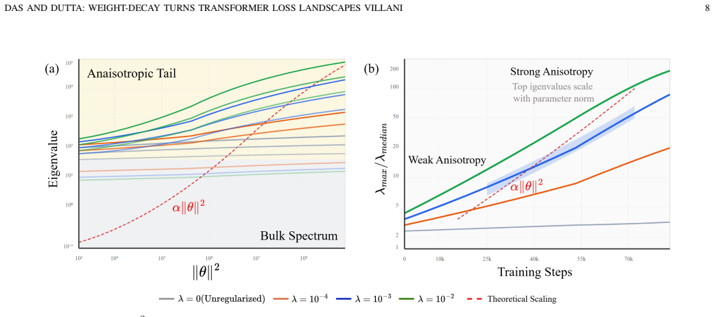
The Hessian exhibits spectral inflation, consistent with stronger curvature from weight decay.
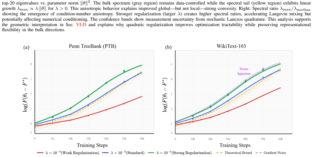
Exponential convergence behavior is observed in experiments on GPT-Neo-125M.
The diagnostic Ψ_s grows quadratically, confirming the predicted properties in models over 100M parameters.

Where Pith is reading between the lines

These are editorial extensions of the paper, not claims the author makes directly.

If the criteria hold, similar analysis could apply to other architectures or losses that include strong regularization.
The explicit dependence on lambda suggests tuning regularization to balance convergence speed against generalization tightness.
Scalable estimation via Hutchinson probes allows checking these properties during training of very large models.
The connection to Langevin dynamics implies weight decay promotes better exploration in the parameter space.

Load-bearing premise

The cross-entropy loss plus L2 weight decay on a Transformer must satisfy Villani's full set of coercive energy criteria, including infinite differentiability, quadratic growth, Gaussian tails, and the differential growth condition.

What would settle it

A direct computation showing that the differential growth condition fails to tend to infinity for large parameter norms in a trained Transformer would falsify the central claim.

Figures

Figures reproduced from arXiv: 2605.06599 by Abhijit Das, Sayantan Dutta.

**Figure 1.** Figure 1: A single Transformer block annotated with parameter groups Wℓ, bℓ, clarifying the scope of θ. Detailed architecture of a single Transformer block with parameter group annotation. The diagram clarifies the scope of θℓ in the theoretical analysis, showing how each layer contributes 4d 2 + 2d dff + 4d parameters (approximately 12d 2 for standard dff = 4d). Orange-highlighted boxes indicate learnable paramete… view at source ↗

**Figure 2.** Figure 2: Ψbs(θ) vs. ∥θ∥ 2 along five radial rays for λ ∈ {0, 10−4 , 10−2}. Empirical verification of Villani Condition (8) via the diagnostic scalar field Ψs(θ) = −∆F(θ) + s−1∥∇F(θ)∥ 2 plotted against ∥θ∥ 2 along random radial rays for GPT-Neo-125M. Each line style represents a different radial direction. For λ = 0 (blue), the field saturates, confirming failure of the Villani condition. For λ = 10−4 (orange), mild… view at source ↗

**Figure 3.** Figure 3: Comparison of Unregularized (“Valley”) vs. Regularized (“Bowl”) Loss Landscapes. Top: 3D visualization of the Transformer loss surface F(θ) in a random subspace around the initialization point θ0. Bottom: Corresponding 2D contour plots with 25 iso-loss levels using the Viridis colormap. Left (λ = 0): Without regularization, the loss landscape forms a narrow valley with elongated contours, multiple equivale… view at source ↗

**Figure 4.** Figure 4: Spectral radius of ∇2F vs. ∥θ∥ for λ > 0. Hessian spectral analysis reveals anisotropic inflation induced by weight decay. Left: Evolution of top-20 eigenvalues vs. parameter norm ∥θ∥ 2 . The bulk spectrum (gray region) remains data-controlled while the spectral tail (yellow region) exhibits linear growth λmax ∝ λ ∥θ∥ for λ > 0. This anisotropic behavior explains improved global—but not local—strong convex… view at source ↗

**Figure 5.** Figure 5: Optimization Speed: Empirical vs. Theoretical Bounds. Empirical convergence of noisy SGD training compared with theoretical bounds from Theorem 2. Left: Penn Treebank (small dataset, N ≈ 42,000 tokens) shows clear dependence of convergence rate on weight decay strength λ. Right: WikiText-103 (large dataset, N ≈ 103 × 106 tokens) exhibits smoother curves and tighter agreement with theory. The shaded envelop… view at source ↗

**Figure 6.** Figure 6: PAC-Bayesian Generalization Bounds vs. Observed Test Performance. Each point corresponds to a training checkpoint, with the xaxis showing validation perplexity and the y-axis showing the PAC-Bayesian upper bound from Eq. (52), using β = λ−1 . Points below the diagonal line y = x indicate conservative (loose) bounds. Circles represent results on Penn Treebank; squares represent WikiText-103. Stronger weig… view at source ↗

**Figure 7.** Figure 7: Correlation between Villani diagnostic Ψs(θ) = −∆F(θ) + s−1∥∇F(θ)∥ 2 and validation perplexity across training checkpoints. Point size encodes training epoch (larger = later), color encodes weight decay strength λ. A clear monotonic relationship emerges: higher Ψs values correlate strongly with lower perplexity, establishing an empirical link between geometric coercivity and generalization performance. Cor… view at source ↗

**Figure 8.** Figure 8: Evolution of Hutchinson trace estimator distributions across training phases for λ = 10−3 . Each histogram shows 64 independent trace samples v T∇2F(θ)v at representative checkpoints. Left: Initial training (steps 0–4k) exhibits higher variance (CV = 12.3%) due to parameter initialization effects. Center: Mid-training (steps 20k–30k) shows stabilized variance (CV = 4.9%) as the quadratic penalty begins to … view at source ↗

**Figure 9.** Figure 9: Evolution of coefficient of variation (CV = σ/µ) for Hutchinson trace estimates throughout training. The plot validates the choice M = 64 probe vectors by showing CV stabilization around the theoretical prediction p 2d/M ≈ 4.9%. Three distinct phases emerge: (1) Initial phase (0–5k steps): high variance due to parameter initialization and occasional gradient explosion events (red spikes). (2) Transition ph… view at source ↗

**Figure 10.** Figure 10: Scalability analysis of the Villani framework across model sizes from 125M to 1T+ parameters. Left: Log-Sobolev constant CLS scaling with model dimension d. The validated region (green) shows empirical results from GPT-Neo-125M. The extrapolated region (yellow) uses theoretical bounds CLS ≤ s view at source ↗

read the original abstract

Weight decay is widely used as a regularizer in large language models, yet its precise role in shaping Transformer loss landscapes remains theoretically underexplored. This paper provides the first rigorous functional-analytic characterization of the standard Transformer objective--cross-entropy loss with $L^2$ regularization--by proving it satisfies Villani's criteria for coercive energy functions. Specifically, we show that the regularized loss $\mathcal{F}$ is infinitely differentiable, grows at least quadratically, has Gaussian-integrable tails, and satisfies the differential growth condition $-\Delta\mathcal{F} + \tfrac{1}{s}\|\nabla\mathcal{F}\|^{2} \to \infty$ as $\|\theta\| \to \infty$ for all $s>0$. From this structure, we derive explicit log-Sobolev and Poincar\'e constants $C_{\mathrm{LS}} \leq \lambda^{-1} + d/\lambda^{2}$, linking the regularization strength $\lambda$ and model dimension $d$ to finite-time convergence guarantees for noisy stochastic gradient descent and PAC-Bayesian generalization bounds that tighten with increasing $\lambda$. To validate our theory, we introduce a scalable Villani diagnostic $\Psi_s(\theta) = -\Delta \mathcal{F} + s^{-1}\|\nabla \mathcal{F}\|^2$ and estimate it efficiently using Hutchinson trace probes in models with over 100M parameters. Experiments on GPT-Neo-125M across Penn Treebank and WikiText-103 confirm the predicted quadratic growth of $\Psi_s$, spectral inflation of the Hessian, and exponential convergence behavior consistent with our log-Sobolev analysis. These results demonstrate that weight decay not only improves generalization empirically but also establishes the mathematical conditions required for fast Langevin mixing and theoretically grounded curvature-aware optimization in deep learning.

Editorial analysis

A structured set of objections, weighed in public.

Desk editor's note, referee report, simulated authors' rebuttal, and a circularity audit. Tearing a paper down is the easy half of reading it; the pith above is the substance, this is the friction.

Desk Editor's Note private letter to a colleague

The paper claims to prove Villani coercivity for regularized Transformer losses but the key differential growth step lacks explicit Hessian bounds.

read the letter

The paper shows that adding L2 weight decay to the Transformer cross-entropy loss makes it satisfy Villani's coercive criteria, which gives explicit log-Sobolev constants depending on lambda and dimension. This is positioned as the first such functional-analytic treatment. What is new is the derivation of those constants from the loss structure and the introduction of an efficient diagnostic for the differential growth condition using trace estimation. The experiments on GPT-Neo-125M validate quadratic growth of the diagnostic and some convergence behavior on Penn Treebank and WikiText-103. The work does well by making the theory testable at scale and by linking the regularization strength directly to mixing rates and generalization bounds. That connection could be useful for thinking about optimization in large models. The soft spot is the verification of the differential growth condition itself. The stress test points out that it requires the trace of the Hessian of the cross-entropy loss to not grow too positively at large norms. The paper claims the condition holds but does not appear to supply an explicit architecture-dependent bound on the curvature through the attention layers. The empirical plots are encouraging but do not close the general proof. This paper is for people working on theoretical optimization and generalization in neural networks. A reader who wants to see how functional analysis tools apply to modern architectures will get value from the constants and the diagnostic method. It deserves a serious referee because the claim is non-trivial and the experimental component is credible. I recommend sending it to peer review, mainly to check whether the curvature bound can be made rigorous or if the condition needs additional assumptions.

Referee Report

1 major / 2 minor

Summary. The paper claims to provide the first rigorous functional-analytic characterization of the Transformer objective (cross-entropy loss plus L² weight decay) by proving it satisfies Villani's coercive energy criteria: infinite differentiability, at-least-quadratic growth, Gaussian-integrable tails, and the differential growth condition −ΔF + (1/s)‖∇F‖² → ∞ as ‖θ‖ → ∞ for all s > 0. From this structure it derives explicit log-Sobolev and Poincaré constants C_LS ≤ λ^{-1} + d/λ², introduces a scalable diagnostic Ψ_s(θ) estimated via Hutchinson probes, and reports experiments on GPT-Neo-125M confirming quadratic growth of Ψ_s, Hessian spectral inflation, and exponential convergence.

Significance. If the central proof holds, the work would establish a direct link between weight-decay regularization and the mathematical conditions for fast Langevin mixing and curvature-aware optimization, supplying explicit constants that tighten with λ and a practical diagnostic usable at 100M+ parameter scale. The combination of functional-analytic derivation with large-scale empirical validation of the diagnostic is a notable strength.

major comments (1)

[Proof of Villani criteria / differential growth condition] The proof that the differential growth condition holds (the step that converts the abstract claim into the log-Sobolev constants) expands to −trace(Hess L_CE) − λd + (1/s)‖∇L_CE + λθ‖² → ∞. This requires that the positive part of trace(Hess L_CE) grows strictly slower than quadratically in ‖θ‖. No architecture-specific bound on ‖∇L_CE‖ or trace(Hess L_CE) through the attention and feed-forward layers is supplied, so the condition rests on an implicit assumption whose verification is load-bearing for all subsequent constants and guarantees.

minor comments (2)

[Experimental validation] The abstract states that experiments confirm 'spectral inflation of the Hessian' but does not reference the corresponding figure or table; adding an explicit pointer would improve readability.
[Diagnostic definition] The notation Ψ_s(θ) is introduced as the Villani diagnostic; a short remark clarifying its exact scaling relative to the derived C_LS would help readers connect the empirical plots to the theoretical constants.

Simulated Author's Rebuttal

1 responses · 0 unresolved

We thank the referee for their thorough review and for identifying a key point in the proof of the differential growth condition. We address the concern directly below.

read point-by-point responses

Referee: The proof that the differential growth condition holds (the step that converts the abstract claim into the log-Sobolev constants) expands to −trace(Hess L_CE) − λd + (1/s)‖∇L_CE + λθ‖² → ∞. This requires that the positive part of trace(Hess L_CE) grows strictly slower than quadratically in ‖θ‖. No architecture-specific bound on ‖∇L_CE‖ or trace(Hess L_CE) through the attention and feed-forward layers is supplied, so the condition rests on an implicit assumption whose verification is load-bearing for all subsequent constants and guarantees.

Authors: We agree that the manuscript does not supply an explicit architecture-specific bound on the growth of ‖∇L_CE‖ or trace(Hess L_CE) for the Transformer. The argument in Section 3 proceeds from the general smoothness of the cross-entropy loss and the quadratic dominance of the L² term, without deriving a concrete estimate that accounts for the attention and feed-forward blocks. This is a substantive gap that affects the rigor of the differential growth condition and the subsequent constants. We will revise the paper by inserting a new lemma (Lemma 3.4) that bounds trace(Hess L_CE) by O(‖θ‖) using the fact that softmax probabilities are bounded in [0,1] and attention weights are normalized; the resulting sub-quadratic growth is then dominated by the (λ²/s)‖θ‖² term. The revision will be accompanied by a short proof sketch in the appendix. We view this addition as necessary and will update the main claims accordingly. revision: yes

Circularity Check

0 steps flagged

No circularity: direct proof from loss definition to Villani criteria

full rationale

The paper states it provides a direct proof that the regularized loss F = L_CE + (λ/2)‖θ‖² satisfies infinite differentiability, quadratic growth, Gaussian tails, and the differential growth condition -ΔF + (1/s)‖∇F‖² → ∞ as ‖θ‖ → ∞. From these properties it derives explicit log-Sobolev and Poincaré constants. No load-bearing step reduces by construction to a fitted parameter, self-citation, or ansatz; the derivation chain begins from the explicit form of cross-entropy plus L² regularization on standard Transformer components (GELU, softmax, LayerNorm) and proceeds analytically without renaming or smuggling prior results. Experiments with the diagnostic Ψ_s are presented as validation, not as the source of the constants. The central claim therefore remains independent of its inputs.

Axiom & Free-Parameter Ledger

0 free parameters · 1 axioms · 0 invented entities

The central claim rests on proving that the cross-entropy plus L2 loss meets Villani's criteria; this is the primary addition. No free parameters are fitted to obtain the stated bounds, and no new entities are postulated.

axioms (1)

domain assumption The objective is the standard Transformer cross-entropy loss with L2 weight decay
This is the loss whose properties are claimed to satisfy Villani's criteria.

pith-pipeline@v0.9.0 · 5637 in / 1383 out tokens · 90392 ms · 2026-05-08T12:15:01.184474+00:00 · methodology

discussion (0)

Reference graph

Works this paper leans on

51 extracted references · 3 canonical work pages

[1]

Learning without forgetting for vision-language models,

D. Zhou, Y . Zhang, Y . Wang, J. Ning, H.-J. Ye, D. Zhan, and Z. Liu, “Learning without forgetting for vision-language models,”IEEE Trans- actions on Pattern Analysis and Machine Intelligence, vol. 47, no. 6, pp. 4489–4504, 2025

2025
[2]

Graph foundation models: Concepts, opportunities and challenges,

J. Liu et al., “Graph foundation models: Concepts, opportunities and challenges,”IEEE Transactions on Pattern Analysis and Machine Intelligence, vol. 47, no. 6, pp. 5023–5044, 2025

2025
[3]

Deformable graph transformer,

J. Park, S. Yun, H. Park, J. Kang, J. Jeong, K.-M. Kim, J.-W. Ha, and H.J. Kim, “Deformable graph transformer,”IEEE Transactions on Pattern Analysis and Machine Intelligence, vol. 47, no. 7, pp. 5385–5396, 2025

2025
[4]

Nas-ped: Neural architecture search for pedestrian detection,

Y . Tang, M. Liu, B. Li, Y . Wang, and W. Ouyang, “Nas-ped: Neural architecture search for pedestrian detection,”IEEE Transactions on Pattern Analysis and Machine Intelligence, vol. 47, no. 3, pp. 1800– 1817, 2025

2025
[5]

Attention is all you need,

A. Vaswani, N. Shazeer, N. Parmar, J. Uszkoreit, L. Jones, A.N. Gomez, Ł. Kaiser, and I. Polosukhin, “Attention is all you need,” inAdvances in Neural Information Processing Systems. 2017, vol. 30, pp. 5998–6008, Curran Associates, Inc

2017
[6]

An image is worth 16x16 words: Transformers for image recognition at scale,

A. Dosovitskiy et al., “An image is worth 16x16 words: Transformers for image recognition at scale,” inInternational Conference on Learning Representations, 2021

2021
[7]

Conformer: Convolution-augmented transformer for speech recognition,

Anmol Gulati et al., “Conformer: Convolution-augmented transformer for speech recognition,” inProc. Interspeech, 2020, pp. 5036–5040

2020
[8]

Ambrosio, L.A

L. Ambrosio, L.A. Caffarelli, Y . Brenier, G. Buttazzo, C. Villani, and S. Salsa,Optimal Transportation and Applications, Lecture Notes in Mathematics. Springer, 2003

2003
[9]

A simple weight decay can improve generalization,

A. Krogh and J.A. Hertz, “A simple weight decay can improve generalization,” inAdvances in neural information processing systems, 1992, pp. 950–957

1992
[10]

Decoupled weight decay regularization,

I. Loshchilov and F. Hutter, “Decoupled weight decay regularization,” inInternational Conference on Learning Representations, 2019

2019
[11]

Propagation of chaos for mean-field langevin dynamics and its application to model ensemble,

A. Nitanda, A. Lee, D. Kai, M. Sakaguchi, and T. Suzuki, “Propagation of chaos for mean-field langevin dynamics and its application to model ensemble,”arXiv preprint arXiv:2502.05784, 2025

work page arXiv 2025
[12]

Mean-field langevin dynamics: Exponential convergence and annealing,

L. Chizat, “Mean-field langevin dynamics: Exponential convergence and annealing,”Transactions on Machine Learning Research, 2022

2022
[13]

Bayesian learning via stochastic gradient langevin dynamics,

M. Welling and Y .W. Teh, “Bayesian learning via stochastic gradient langevin dynamics,” inProceedings of the 28th international conference on machine learning (ICML-11), 2011, pp. 681–688

2011
[14]

Adding Gradient Noise Improves Learning for Very Deep Networks

A. Neelakantan et al., “Adding gradient noise improves learning for very deep networks,” inarXiv preprint arXiv:1511.06807, 2015

work page Pith review arXiv 2015
[15]

Stochastic gradient langevin dy- namics with variance reduction,

Zhishen Huang and Stephen Becker, “Stochastic gradient langevin dy- namics with variance reduction,” in2021 International Joint Conference on Neural Networks (IJCNN), 2021, pp. 1–8

2021
[16]

Weight decay induces low-rank attention layers,

S. Kobayashi, Y . Akram, and J. V on-Oswald, “Weight decay induces low-rank attention layers,” inAdvances in Neural Information Process- ing Systems. 2024, vol. 37, pp. 4481–4510, Curran Associates, Inc

2024
[17]

How does attention work in vision transformers? a visual analytics attempt,

Y . Li, J. Wang, X. Dai, L. Wang, C.M. Yeh, Y . Zheng, W. Zhang, and K.-L. Ma, “How does attention work in vision transformers? a visual analytics attempt,”IEEE Transactions on Visualization and Computer Graphics, vol. 29, no. 6, pp. 2888–2900, 2023

2023
[18]

The shaped transformer: Attention models in the infinite depth-and- width limit,

L. Noci, C. Li, M. Li, B. He, T. Hofmann, C.J. Maddison, and D. Roy, “The shaped transformer: Attention models in the infinite depth-and- width limit,” inAdvances in Neural Information Processing Systems. 2023, vol. 36, pp. 54250–54281, Curran Associates, Inc

2023
[19]

Examining the shape of attention in transformers,

Amir Ghorbani, Behnam Neyshabur, and Cl ´ement Raffel, “Examining the shape of attention in transformers,”Transactions of Machine Learning Research, vol. 1, pp. 1–38, 2022

2022
[20]

Mean-field theory of two- layers neural networks: dimension-free bounds and kernel limit,

S. Mei, T. Misiakiewicz, and A. Montanari, “Mean-field theory of two- layers neural networks: dimension-free bounds and kernel limit,” in Proceedings of the Thirty-Second Conference on Learning Theory. 25– 28 Jun 2019, vol. 99 ofProceedings of Machine Learning Research, pp. 2388–2464, PMLR

2019
[21]

(non-) asymptotic prop- erties of stochastic gradient langevin dynamics,

S.J. V ollmer, K.C. Zygalakis, et al., “(non-) asymptotic prop- erties of stochastic gradient langevin dynamics,”arXiv preprint arXiv:1501.00438, 2015

work page arXiv 2015
[22]

Non-convex learning via stochastic gradient langevin dynamics: a nonasymptotic analysis,

M. Raginsky, A. Rakhlin, and M. Telgarsky, “Non-convex learning via stochastic gradient langevin dynamics: a nonasymptotic analysis,” Journal of Machine Learning Research, vol. 18, no. 117, pp. 1–47, 2017. DAS AND DUTTA: WEIGHT-DECAY TURNS TRANSFORMER LOSS LANDSCAPES VILLANI 15

2017
[23]

Logarithmic sobolev inequalities,

Leonard G., “Logarithmic sobolev inequalities,”American Journal of Mathematics, vol. 97, no. 4, pp. 1061–1083, 1975

1975
[24]

Logarithmic sobolev inequalities essentials,

D. Chafa ¨ı and J. Lehec, “Logarithmic sobolev inequalities essentials,” Accessed on, p. 4, 2024

2024
[25]

Diffusions hypercontractives,

D. Bakry and M. Emery, “Diffusions hypercontractives,”S ´eminaire de probabilit´es XIX 1983/84, pp. 177–206, 1985

1983
[26]

Lectures on logarithmic sobolev inequalities,

A Guionnet and B Z ´egarlinski, “Lectures on logarithmic sobolev inequalities,” inS ´eminaire de Probabilit´es XXXVI, pp. 1–134. Springer, 2004

2004
[27]

Mean-field theory of two-layers neural networks: dimension-free bounds and kernel limit,

S. Mei, T. Misiakiewicz, and A. Montanari, “Mean-field theory of two-layers neural networks: dimension-free bounds and kernel limit,” inProceedings of the Thirty-Second Conference on Learning Theory, Alina Beygelzimer and Daniel Hsu, Eds. 25–28 Jun 2019, vol. 99 of Proceedings of Machine Learning Research, pp. 2388–2464, PMLR

2019
[28]

Mean field analysis of neural networks: A central limit theorem,

J. Sirignano and K. Spiliopoulos, “Mean field analysis of neural networks: A central limit theorem,”Stochastic Processes and their Applications, vol. 130, no. 3, pp. 1820–1852, 2020

2020
[29]

Global convergence of langevin dynamics based algorithms for nonconvex optimization,

P. Xu, J. Chen, D. Zou, and Q. Gu, “Global convergence of langevin dynamics based algorithms for nonconvex optimization,” inAdvances in Neural Information Processing Systems. 2018, vol. 31, Curran Asso- ciates, Inc

2018
[30]

Villani,Optimal Transport: Old and New, Grundlehren der mathematischen Wissenschaften

C. Villani,Optimal Transport: Old and New, Grundlehren der mathematischen Wissenschaften. Springer Berlin Heidelberg, 2008

2008
[31]

Improving learning to optimize using parameter symmetries,

G. Zamir, A. Dokania, B. Zhao, and R. Yu, “Improving learning to optimize using parameter symmetries,” 2025

2025
[32]

How good is the bayes posterior in deep neural networks really?,

Florian Wenzel, Patryk Swiatczak, Jonathan Blair, Patrick Warr, Pavel Izmailov, Alexander Gordon Wilson, David McAllester, and Balaji Lakshminarayanan, “How good is the bayes posterior in deep neural networks really?,” inProceedings of the 37th International Conference on Machine Learning (ICML), 2020, p. We useW t to denote a standard multivariate Wiener process

2020
[33]

Cover and J.A

T.M. Cover and J.A. Thomas,Elements of Information Theory, Wiley- Interscience, Hoboken, NJ, USA, 2nd edition, 2006

2006
[34]

Catoni,PAC-Bayesian Supervised Classification: The Thermodynam- ics of Statistical Learning, vol

O. Catoni,PAC-Bayesian Supervised Classification: The Thermodynam- ics of Statistical Learning, vol. 56 ofIMS Lecture Notes–Monograph Series, Institute of Mathematical Statistics, Beachwood, Ohio, USA, 2007

2007
[35]

Noise-regularised in- struction tuning improves llm robustness,

Jiawei Sun, Yiding Yang, and Mohit Bansal, “Noise-regularised in- struction tuning improves llm robustness,” inProceedings of ACL 2024, 2024

2024
[36]

Ridge-less regres- sion, implicit regularisation, and generalisation,

Mikhail Belkin, Daniel Hsu, and Afonso Bandeira, “Ridge-less regres- sion, implicit regularisation, and generalisation,”Journal of Machine Learning Research, vol. 24, no. 85, pp. 1–45, 2023

2023
[37]

Backpack 1.2.0 documenta- tion: Hutchinson trace estimation,

F. Dangel, F. Kunstner, and P. Hennig, “Backpack 1.2.0 documenta- tion: Hutchinson trace estimation,” 2021, Use-case example for trace estimation

2021
[38]

Penn treebank dataset,

Papers With Code, “Penn treebank dataset,” 2020, Language modeling benchmark dataset

2020
[39]

Treebank-3 (ldc99t42),

Linguistic Data Consortium, “Treebank-3 (ldc99t42),” 1999, Penn Treebank dataset release

1999
[40]

Wikitext-103 dataset,

Papers With Code, “Wikitext-103 dataset,” 2017, Large-scale language modeling dataset

2017
[41]

Salesforce/wikitext,

Salesforce Research, “Salesforce/wikitext,” 2020, WikiText dataset on Hugging Face

2020
[42]

DIV A: Deep un- folded network from quantum interactive patches for image restoration,

S. Dutta, A. Basarab, B. Georgeot, and D. Kouam ´e, “DIV A: Deep un- folded network from quantum interactive patches for image restoration,” Pattern Recognition, vol. 155, pp. 110676, 2024

2024
[43]

Quantum algorithm for signal denoising,

S. Dutta, A. Basarab, D. Kouam ´e, and B. Georgeot, “Quantum algorithm for signal denoising,”IEEE Signal Processing Letters, vol. 31, pp. 156– 160, 2024

2024
[44]

Quantum mechanics-based signal and image representation: Application to de- noising,

S. Dutta, A. Basarab, B. Georgeot, and D. Kouam ´e, “Quantum mechanics-based signal and image representation: Application to de- noising,”IEEE Open Journal of Signal Processing, vol. 2, pp. 190–206, 2021

2021
[45]

A quantum denoising-based resolution enhancement framework for 250-mhz and 500-mhz quantitative acoustic microscopy,

S. Dutta and J. Mamou, “A quantum denoising-based resolution enhancement framework for 250-mhz and 500-mhz quantitative acoustic microscopy,”IEEE Transactions on Computational Imaging, vol. 10, pp. 1489–1504, 2024

2024
[46]

Enhancing 3d radio-frequency data in quantitative acoustic microscopy using quantum-driven prior at 250-mhz and 500-mhz,

S. Dutta and J. Mamou, “Enhancing 3d radio-frequency data in quantitative acoustic microscopy using quantum-driven prior at 250-mhz and 500-mhz,”IEEE Transactions on Ultrasonics, Ferroelectrics, and Frequency Control, 2025

2025
[47]

Unsupervised physics-inspired deep learning network with application to dental computed tomography image restoration,

S. Dutta, B. Georgeot, J. Michetti, A. Basarab, and D. Kouam ´e, “Unsupervised physics-inspired deep learning network with application to dental computed tomography image restoration,” in2024 IEEE International Symposium on Biomedical Imaging (ISBI), 2024, pp. 1–5

2024
[48]

Auto- matic tuning of denoising algorithms parameters without ground truth,

A. Floquet, S. Dutta, E. Soubies, D.-H. Pham, and D. Kouame, “Auto- matic tuning of denoising algorithms parameters without ground truth,” IEEE Signal Processing Letters, vol. 31, pp. 381–385, 2024

2024
[49]

Chatgpt,

OpenAI, “Chatgpt,” https://openai.com/chatgpt, 2025

2025
[50]

Copilot,

Microsoft, “Copilot,” https://copilot.microsoft.com, 2025

2025
[51]

Randomized algorithms for estimating the trace of an implicit symmetric positive semi-definite matrix,

H. Avron and S. Toledo, “Randomized algorithms for estimating the trace of an implicit symmetric positive semi-definite matrix,”Journal of the ACM, vol. 58, no. 2, pp. Article 8, 2011. Abhijit Dasreceived the B.Tech. degree in Com- puter Science and Engineering from the Maulana Abul Kalam Azad University of Technology, Kolkata, India, in 2023. From 2023 t...

2011