Recognition: no theorem link
Physics-Based Flow Matching for Full-Field Prediction of Silicon Photonic Devices
Pith reviewed 2026-05-11 00:56 UTC · model grok-4.3
The pith
A conditional flow matching model with physics constraints predicts full electromagnetic field distributions in silicon photonic devices from geometry and wavelength.
A machine-rendered reading of the paper's core claim, the machinery that carries it, and where it could break.
Core claim
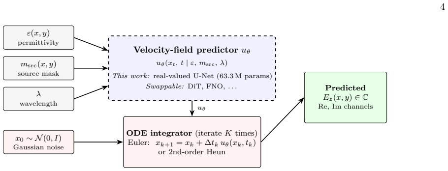
PIC-Flow is a generative neural surrogate that predicts electromagnetic field distributions for photonic devices given their geometry and operating wavelength. It combines conditional flow matching as the generative framework, a real-valued U-Net operating on split real and imaginary field channels, and physics-constrained training through a Helmholtz residual loss with an interface-aware masking scheme that excludes dielectric boundary pixels.
What carries the argument
Conditional flow matching that learns a velocity field transporting Gaussian noise to physically valid field solutions, guided by the masked Helmholtz residual enforcing the wave equation away from interfaces.
If this is right
- The surrogate enables rapid design-space exploration of photonic integrated circuits by replacing repeated FDTD runs with fast neural inference.
- With broader data coverage, more compute, and further optimization the approach could scale toward broadband, device-agnostic field prediction.
- Dramatically reduced runtime supports iterative design of complex photonic devices and circuits.
- Generalization to unseen device classes like S-bends and cascaded Y-branches demonstrates the model's potential beyond the training distribution.
Where Pith is reading between the lines
- The strong physics constraint could reduce the amount of FDTD training data needed compared with purely data-driven surrogates.
- Integration into inverse-design loops would allow geometry optimization directly in field space without repeated full simulations.
- Extension to three-dimensional or broadband problems would require adapting the masking scheme and expanding the training distribution.
Load-bearing premise
The interface-aware masking scheme for the Helmholtz residual excludes only dielectric boundary pixels where finite-difference errors dominate without removing critical physics information or failing to generalize across device types.
What would settle it
On a held-out device class the predicted fields show large violations of the Helmholtz equation in interior regions, or the surrogate fails to match FDTD accuracy on new geometries while runtime gains are measured.
Figures


read the original abstract
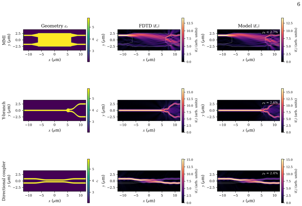
Designing photonic integrated circuits requires accurate electromagnetic field simulations, which remain computationally expensive even for simple device geometries. We present PIC-Flow, a generative neural surrogate that predicts electromagnetic field distributions for photonic devices given their geometry and operating wavelength as an alternative to costly finite-difference time-domain (FDTD) simulations. Our approach combines three key ideas: (i) conditional flow matching as the generative framework, learning a velocity field that transports Gaussian noise to physically valid field solutions; (ii) a real-valued U-Net operating on split real and imaginary field channels; and (iii) physics-constrained training through a Helmholtz residual loss enforcing $\nabla^2 E_z + k_0^2 \varepsilon E_z = 0$. We introduce an interface-aware masking scheme for the Helmholtz residual that excludes dielectric boundary pixels where finite-difference stencil errors dominate, yielding a physically meaningful compliance metric. The data set consists of 22,500 ground-truth FDTD simulations split evenly between multimode interferometers, Y-branches, and directional couplers at $\lambda=1.55\,\mu$m in an 80/10/10 split between training, validation, and test sets. We evaluate ablations on the network against the held out test devices and also show that the model generalizes to held out device classes such as S-bends, tapers, and cascaded Y-branches. Rather than a drop-in replacement for FDTD, this work establishes a foundation that, with broader data coverage, more compute, and further training optimization, could scale toward broadband, device-agnostic field prediction with dramatically improved runtime for rapid design-space exploration of complex photonic devices and circuits.
Editorial analysis
A structured set of objections, weighed in public.
Referee Report
Summary. The manuscript introduces PIC-Flow, a conditional flow-matching generative model based on a real-valued U-Net that predicts full electromagnetic field distributions (split real/imaginary channels) for silicon photonic devices given geometry and wavelength. It augments standard flow-matching training with a physics-constrained Helmholtz residual loss, using an interface-aware mask that excludes dielectric boundary pixels, and is trained on 22,500 FDTD simulations of MMIs, Y-branches, and directional couplers. The work reports ablations on held-out test devices and generalization to unseen classes such as S-bends, tapers, and cascaded Y-branches.
Significance. If the predictions prove accurate and physically consistent, the approach could enable rapid design-space exploration in photonic integrated circuits by replacing expensive FDTD runs with fast neural surrogates. The combination of flow matching with a masked physics residual is a timely contribution to surrogate modeling in nanophotonics.
major comments (2)
- [Abstract] Abstract (physics-constrained training paragraph): the interface-aware masking scheme excludes dielectric boundary pixels from the Helmholtz residual loss because finite-difference stencils are inaccurate there. These same pixels encode the index discontinuities that govern confinement, scattering, and mode matching. No alternative enforcement of interface conditions (e.g., explicit continuity or higher-order stencils) is described, so nothing in the loss prevents non-physical jumps or incorrect evanescent tails at the locations that matter most for device behavior.
- [Abstract] Abstract (evaluation paragraph): the manuscript states that ablations were performed against held-out test devices and that generalization to S-bends, tapers, and cascaded Y-branches was shown, yet no quantitative error metrics (MSE, field correlation, power conservation error), baseline comparisons, or ablation tables appear. Without these numbers the central performance and generalization claims cannot be assessed.
minor comments (2)
- The abstract mentions an 80/10/10 split of the 22,500 simulations but does not state the exact number of geometries per device class or the range of geometric parameters sampled.
- Clarify how the geometry and wavelength are encoded as conditioning inputs to the U-Net (e.g., channel concatenation, embedding).
Simulated Author's Rebuttal
We thank the referee for their constructive and detailed feedback on our manuscript. We have addressed each major comment point by point below, providing clarifications and committing to revisions that strengthen the presentation of our physics-constrained approach and evaluation results.
read point-by-point responses
-
Referee: [Abstract] Abstract (physics-constrained training paragraph): the interface-aware masking scheme excludes dielectric boundary pixels from the Helmholtz residual loss because finite-difference stencils are inaccurate there. These same pixels encode the index discontinuities that govern confinement, scattering, and mode matching. No alternative enforcement of interface conditions (e.g., explicit continuity or higher-order stencils) is described, so nothing in the loss prevents non-physical jumps or incorrect evanescent tails at the locations that matter most for device behavior.
Authors: We appreciate the referee highlighting this subtlety in our physics-informed loss. The interface-aware mask is applied specifically because the second-order finite-difference stencil for the Laplacian is known to produce large errors at permittivity discontinuities; including those pixels would contaminate the residual with numerical artifacts rather than physical violations. The training data, however, are full-wave FDTD solutions that correctly satisfy the electromagnetic interface conditions (continuity of tangential E and normal D). The conditional flow-matching model therefore learns the correct field behavior at boundaries directly from data, while the masked Helmholtz term enforces the wave equation only in the homogeneous interior regions. We agree that an explicit interface term would be desirable and will revise the Methods section to (i) clarify the complementary roles of data-driven learning and the masked residual, (ii) acknowledge the current limitation, and (iii) outline planned extensions using higher-order or interface-specific penalties. revision: yes
-
Referee: [Abstract] Abstract (evaluation paragraph): the manuscript states that ablations were performed against held-out test devices and that generalization to S-bends, tapers, and cascaded Y-branches was shown, yet no quantitative error metrics (MSE, field correlation, power conservation error), baseline comparisons, or ablation tables appear. Without these numbers the central performance and generalization claims cannot be assessed.
Authors: The referee is correct that the abstract itself contains only a high-level summary. The full manuscript reports the requested quantitative results in the Experiments and Results sections: ablation tables list MSE, field Pearson correlation, and integrated power-conservation error on the held-out test split; baseline comparisons against a non-physics-informed U-Net and a standard conditional diffusion model are provided; and generalization performance on S-bends, tapers, and cascaded Y-branches is quantified with per-class error metrics and example field visualizations. To make these claims immediately verifiable from the abstract, we will revise the evaluation paragraph to include representative numerical values (e.g., mean test-set MSE and correlation) and will ensure the abstract explicitly references the supporting tables and figures. revision: yes
Circularity Check
No significant circularity; derivation relies on external data and independent constraint
full rationale
The paper trains a conditional flow-matching model on independent FDTD ground-truth simulations of device geometries and augments training with a Helmholtz residual loss. The interface-aware masking is a deliberate design choice in the loss term rather than a definitional loop, and the generated fields are not equivalent to the inputs by construction; the model must learn a velocity field from noise conditioned on geometry and wavelength. Generalization results on held-out device classes (S-bends, tapers, cascaded Y-branches) provide an external check against pure data fitting. No self-citations, uniqueness theorems, or fitted parameters renamed as predictions appear as load-bearing elements in the derivation chain.
Axiom & Free-Parameter Ledger
free parameters (1)
- U-Net architecture and training hyperparameters
axioms (1)
- domain assumption Time-harmonic electromagnetic fields inside the devices obey the source-free Helmholtz equation ∇²E_z + k₀² ε E_z = 0 away from material interfaces.
Reference graph
Works this paper leans on
-
[1]
U-Net architecture The architecture follows the standard encoder– bottleneck–decoder layout with skip connections, resid- ual blocks, and attention at selected spatial resolutions. a. Residual convolutional blocks.Each resolution level contains convolutional residual blocks with normal- ization, nonlinear activation, and dropout. Downsam- pling in the enc...
-
[2]
The first is the explicit (first-order) Euler step xk+1 =x k + ∆tk ˆuθ(xk, tk),(A1) which requires a single network evaluation per step and is what the wall-clock benchmark in Sec
Inference integrators We integrate the learned velocity field fromt= 0 (Gaussian noise) tot= 1 on a linear time grid using one of two integrators. The first is the explicit (first-order) Euler step xk+1 =x k + ∆tk ˆuθ(xk, tk),(A1) which requires a single network evaluation per step and is what the wall-clock benchmark in Sec. VI C uses. The second is the ...
-
[3]
The training tensors are cropped/resampled to a 160×480 grid atdx=dy= 0.05µm
FDTD simulation parameters Meep simulations use an eigenmode source exciting the fundamental TE mode at the selected input port, run until field energy decays below a convergence threshold (typically seconds to minutes per geometry on CPU). The training tensors are cropped/resampled to a 160×480 grid atdx=dy= 0.05µm. Per simulation we store the complex fi...
-
[4]
Without phase anchoring, the same device at the same wavelength could produce training targets with different global phases, preventing the model from learning a consistent mapping
Phase anchoring Frequency-domain fields have an arbitrary global phase, meaning that ifE z is a solution to the Helmholtz equation, so isE zeiϕ. Without phase anchoring, the same device at the same wavelength could produce training targets with different global phases, preventing the model from learning a consistent mapping. We anchor the global phase usi...
-
[5]
All mea- surements are taken on the same compute node: an NVIDIA A100 GPU paired with dual AMD EPYC 75F3 processors (2×32 physical cores, Zen3)
Wall-clock benchmark configuration The wall-clock comparison in Section VI C is per- formed on a single held-out directional coupler (gap = 0.175µm,L c = 5.97µm,λ= 1.55µm). All mea- surements are taken on the same compute node: an NVIDIA A100 GPU paired with dual AMD EPYC 75F3 processors (2×32 physical cores, Zen3). FDTD is run with Meep on 16 threads, in...
-
[6]
C. Sun, M. T. Wade, Y. Lee, J. S. Orcutt, L. Alloatti, M. S. Georgas, A. S. Waterman, J. M. Shainline, R. R. Avizienis, S. Lin,et al., Nature528, 534 (2015)
2015
-
[7]
Rizzo, A
A. Rizzo, A. Novick, V. Gopal, B. Y. Kim, X. Ji, S. Daudlin, Y. Okawachi, Q. Cheng, M. Lipson, A. L. Gaeta,et al., Nature Photonics17, 781 (2023)
2023
-
[8]
Daudlin, A
S. Daudlin, A. Rizzo, S. Lee, D. Khilwani, C. Ou, S. Wang, A. Novick, V. Gopal, M. Cullen, R. Parsons, et al., Nature Photonics19, 502 (2025)
2025
-
[9]
Rogers, A
C. Rogers, A. Y. Piggott, D. J. Thomson, R. F. Wiser, I. E. Opris, S. A. Fortune, A. J. Compston, A. Gondarenko, F. Meng, X. Chen,et al., Nature590, 256 (2021)
2021
-
[10]
K. D. Vos, I. Bartolozzi, E. Schacht, P. Bienstman, and R. Baets, Optics express15, 7610 (2007)
2007
-
[11]
M. Yu, Y. Okawachi, A. G. Griffith, N. Picqu´ e, M. Lip- son, and A. L. Gaeta, Nature communications9, 1869 (2018)
2018
-
[12]
S. R. Ahmed, R. Baghdadi, M. Bernadskiy, N. Bow- man, R. Braid, J. Carr, C. Chen, P. Ciccarella, M. Cole, J. Cooke,et al., Nature640, 368 (2025)
2025
-
[13]
S. Hua, E. Divita, S. Yu, B. Peng, C. Roques-Carmes, Z. Su, Z. Chen, Y. Bai, J. Zou, Y. Zhu,et al., Nature 640, 361 (2025)
2025
-
[14]
Bandyopadhyay, A
S. Bandyopadhyay, A. Sludds, S. Krastanov, R. Hamerly, N. Harris, D. Bunandar, M. Streshinsky, M. Hochberg, and D. Englund, Nature Photonics18, 1335 (2024)
2024
-
[15]
Taflove and S
A. Taflove and S. C. Hagness,Computational Electro- dynamics: The Finite-Difference Time-Domain Method, 3rd ed. (Artech House, 2005)
2005
-
[16]
F. L. Teixeira, C. Sarris, Y. Zhang, D.-Y. Na, J.- P. Berenger, Y. Su, M. Okoniewski, W. C. Chew, V. Backman, and J. J. Simpson, Nature Reviews Meth- ods Primers3, 75 (2023)
2023
-
[17]
Flow Matching for Generative Modeling
Y. Lipman, R. T. Chen, H. Ben-Hamu, M. Nickel, and M. Le, Flow matching for generative modeling (2022), arXiv:2210.02747 [cs.LG]
work page internal anchor Pith review Pith/arXiv arXiv 2022
-
[18]
Flow matching meets PDE s: A unified framework for physics-constrained generation
G. Baldan, Q. Liu, A. Guardone, and N. Thuerey, Physics vs distributions: Pareto optimal flow matching with physics constraints (2025), arXiv:2506.08604 [cs.LG]
-
[19]
Jiang, M
J. Jiang, M. Chen, and J. A. Fan, Nature Reviews Ma- terials6, 679 (2021)
2021
-
[20]
W. Ma, Z. Liu, Z. A. Kudyshev, A. Boltasseva, W. Cai, and Y. Liu, Nature Photonics15, 77 (2021)
2021
-
[21]
M. H. Tahersima, K. Kojima, T. Koike-Akino, D. Jha, B. Wang, C. Lin, and K. Parsons, Scientific Reports9, 1368 (2019)
2019
-
[22]
Y. Tang, K. Kojima, T. Koike-Akino, Y. Wang, P. Wu, Y. Xie, M. H. Tahersima, D. K. Jha, K. Parsons, and M. Qi, Laser & Photonics Reviews14, 2000287 (2020)
2020
-
[23]
Ronneberger, P
O. Ronneberger, P. Fischer, and T. Brox, inMedical Image Computing and Computer-Assisted Intervention (MICCAI), Lecture Notes in Computer Science, Vol. 9351 (Springer, 2015) pp. 234–241
2015
-
[24]
M. Chen, R. Lupoiu, C. Mao, D.-H. Huang, J. Jiang, P. Lalanne, and J. A. Fan, ACS Photonics9, 3110 (2022)
2022
-
[25]
Lim and D
J. Lim and D. Psaltis, APL Photonics7, 011301 (2022)
2022
-
[26]
Raissi, P
M. Raissi, P. Perdikaris, and G. E. Karniadakis, Journal of Computational Physics378, 686 (2019)
2019
-
[27]
Z. Li, N. Kovachki, K. Azizzadenesheli, B. Liu, K. Bhat- tacharya, A. Stuart, and A. Anandkumar, Fourier neu- ral operator for parametric partial differential equations (2020), arXiv:2010.08895 [cs.LG]
work page internal anchor Pith review Pith/arXiv arXiv 2020
-
[28]
L. Lu, P. Jin, G. Pang, Z. Zhang, and G. E. Karniadakis, Nature Machine Intelligence3, 218 (2021)
2021
-
[29]
Y. Song, J. Sohl-Dickstein, D. P. Kingma, A. Kumar, S. Ermon, and B. Poole, inInternational Conference on Learning Representations (ICLR)(2021)
2021
-
[30]
Huang, G
J. Huang, G. Yang, Z. Wang, and J. J. Park, inAdvances in Neural Information Processing Systems (NeurIPS), Vol. 37 (2024) pp. 130291–130323
2024
-
[31]
Molesky, Z
S. Molesky, Z. Lin, A. Y. Piggott, W. Jin, J. Vuˇ ckovi´ c, and A. W. Rodriguez, Nature Photonics12, 659 (2018)
2018
-
[32]
A. Y. Piggott, J. Lu, K. G. Lagoudakis, J. Petykiewicz, T. M. Babinec, and J. Vuˇ ckovi´ c, Nature Photonics9, 374 (2015)
2015
-
[33]
A. Y. Piggott, J. Petykiewicz, L. Su, and J. Vuˇ ckovi´ c, Scientific Reports7, 1786 (2017)
2017
-
[34]
Yeung, B
C. Yeung, B. Pham, R. Tsai, K. T. Fountaine, and A. P. Raman, ACS Photonics10, 884 (2023)
2023
-
[35]
Pan and X
Z. Pan and X. Pan, Photonics10, 852 (2023)
2023
-
[36]
G. T. Reed and A. P. Knights,Silicon Photonics: An Introduction(John Wiley & Sons, 2004)
2004
-
[37]
X. Liu, C. Gong, and Q. Liu, inInternational Conference on Learning Representations (ICLR)(2023)
2023
-
[38]
A. F. Oskooi, D. Roundy, M. Ibanescu, P. Bermel, J. D. Joannopoulos, and S. G. Johnson, Computer Physics Communications181, 687 (2010)
2010
-
[39]
G. W. Burr and A. Farjadpour, inProceedings of SPIE, Vol. 5733 (2005) pp. 336–347
2005
discussion (0)
Sign in with ORCID, Apple, or X to comment. Anyone can read and Pith papers without signing in.