Recognition: no theorem link
Characterizing the Extended Molecular Hydrogen Winds in Protoplanetary Disks from the JWST Disk Infrared Spectroscopic Chemistry Survey
Pith reviewed 2026-05-11 01:09 UTC · model grok-4.3
The pith
Molecular winds traced by H2 emission can disperse typical protoplanetary disks in 2-3 million years.
A machine-rendered reading of the paper's core claim, the machinery that carries it, and where it could break.
Core claim
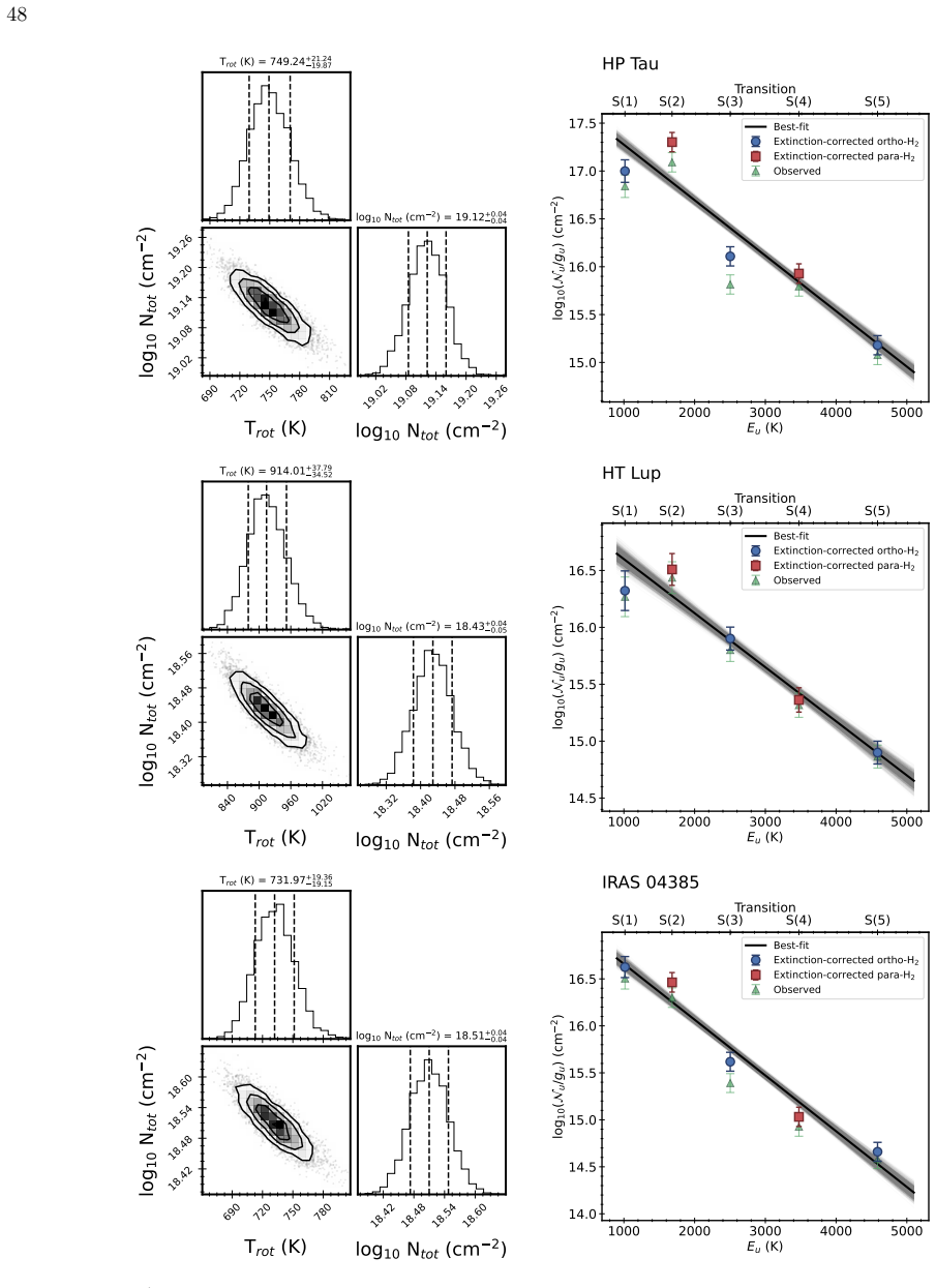
Extended H2 emission is common in protoplanetary disks and traces wide-angle molecular winds driven by MHD processes at velocities of about 4 km/s. For ten disks, morphological modeling gives a median half-opening angle of 45 degrees and density power-law index of 1.6, with excitation conditions showing median temperatures of 624 K and total column densities of 10^18.6 cm^{-2}. The resulting wind mass-loss rates cluster tightly around a median log10 value of -9 solar masses per year, indicating that these winds alone could account for the dispersal of typical 2-3 Jupiter-mass disks within 2-3 Myr, consistent with empirical disk lifetimes, while showing little direct correlation with stellar
What carries the argument
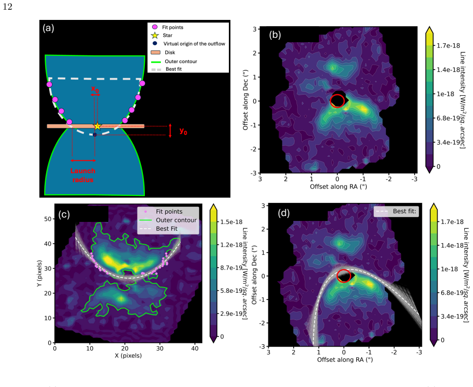
Spatially extended pure rotational H2 emission modeled as wide-angle disk winds using half-opening angles near 45 degrees and power-law density profiles to convert line fluxes into total mass-loss rates.
If this is right
- Molecular winds traced by H2 represent a widespread disk dispersal channel operating across many systems.
- Typical disks reach dispersal in 2-3 Myr when wind mass loss dominates.
- Wind mass-loss rates occupy a narrow range of roughly 2 dex and remain decoupled from stellar accretion rates.
- H2 lines serve as reliable tracers for both inclined and face-on wind geometries.
Where Pith is reading between the lines
- Disk evolution models may need to incorporate MHD wind mass loss as a primary channel alongside photoevaporation.
- Higher-resolution spectroscopy could map wind launching radii and test whether the narrow rate distribution holds for larger samples.
- The decoupling from accretion rates suggests that wind-driven dispersal and stellar accretion probe distinct evolutionary phases or episodic behaviors.
Load-bearing premise
The spatially extended H2 emission originates from disk winds rather than other kinematic components and the adopted wind morphology models accurately convert the observed fluxes into total mass-loss rates.
What would settle it
A direct measurement or alternative tracer showing that the H2 emission arises from bound disk gas or non-wind flows, or a median wind mass-loss rate differing by more than an order of magnitude from 10^{-9} solar masses per year.
Figures


read the original abstract
We present a comprehensive analysis of extended H$_2$ emission from 34 protoplanetary disks observed with the JWST Disk Infrared Spectroscopic Chemistry Survey (JDISCS), supplemented by archival data. We investigated the morphology, kinematics, excitation conditions, and mass dynamics of H$_2$. Extended emission from pure rotational H$_2$ lines is found to be common, with 16 sources exhibiting clear signatures of disk winds. These include monopolar and bipolar structures in inclined disks and ring-like or bubble-like morphologies in face-on systems features indicative of wide-angle disk winds. Our analysis shows that the H$_2$ is consistent with slow {(4.2$^{+6.7}_{-3.0}$ km s$^{-1}$)} MHD driven winds. For ten disks, we model the wind morphology and find a median half-opening angle of $45\arcdeg^{+5}_{-4}$ and a characteristic power-law index of $\alpha \sim$ 1.6. Excitation analysis yields a median gas temperature of 624 $\pm$ 130 K and a column density of $\log(N_{\mathrm{tot}}\,[\mathrm{cm}^{-2}]) = 18.6 \pm 0.6$. The median wind mass-loss rate, ${\rm log_{10}}(\dot{\rm M}_{\rm wind}^{\rm tot}) = -9_{-0.4}^{+0.8}\,{\rm M_\odot\,yr^{-1}}$, implies that, if molecular winds are the dominant mechanism responsible for disk dispersal, a typical disk with a mass of $2-3\,M_{\rm Jup}$ would dissipate on a $\sim$2-3 Myr timescale, consistent with observed disk lifetimes. The $\dot{\rm M}_{\mathrm{\rm wind}}^{\rm tot}$ span a relatively narrow range ($\sim$2 dex) and do not correlate strongly with accretion rates onto the star, suggesting that the mass loss rate and the accretion rates are probing different timescales. Our findings demonstrate that spatially extended warm H$_2$ emission is a widespread and reliable tracer of molecular disk winds in protoplanetary systems.
Editorial analysis
A structured set of objections, weighed in public.
Referee Report
Summary. The manuscript analyzes extended pure-rotational H2 emission in 34 protoplanetary disks from the JWST JDISCS survey (plus archival data). It reports clear wind signatures in 16 sources, including monopolar/bipolar structures and ring/bubble morphologies. For ten disks, wind morphology is modeled with a median half-opening angle of 45°+5−4 and power-law index α∼1.6; excitation analysis yields median T=624±130 K and log N_tot=18.6±0.6. The resulting median log10(Ṁ_wind^tot)=−9−0.4+0.8 M⊙ yr−1 is used to argue that molecular winds can disperse a typical 2–3 MJup disk in ∼2–3 Myr, consistent with observed lifetimes. The rates span ∼2 dex and show no strong correlation with stellar accretion rates, supporting slow MHD winds as a widespread dispersal mechanism.
Significance. If the mass-loss rates prove robust, the work supplies one of the largest observational samples of molecular disk winds to date and directly links JWST-detected H2 structures to disk-evolution timescales. The narrow range of Ṁ values and the decoupling from accretion rates are potentially important constraints on wind-launching physics. The survey-scale detection statistics strengthen the case that extended warm H2 is a reliable wind tracer.
major comments (2)
- [Wind morphology modeling for the ten disks (values and assumptions stated in the abstract and corresponding analysis)] The headline implication (2–3 Myr dissipation for a 2–3 MJup disk) rests on the median log10(Ṁ_wind^tot)=−9 reported for the ten modeled sources. This value is obtained only after fixing the half-opening angle at 45°+5−4 and the density power-law index at α∼1.6 to convert observed line fluxes into total mass-loss rates. No sensitivity analysis quantifies how Ṁ (and therefore the timescale) changes when these parameters are varied within plausible ranges or when the wind is allowed to be narrower or steeper.
- [Kinematic and morphological classification of the 16 wind sources] The claim that the spatially extended H2 traces disk winds (rather than bound Keplerian emission, shocks, or other kinematic components) is central to interpreting all 16 detections and the derived Ṁ values. While morphologies are described as “indicative of wide-angle winds,” the manuscript does not present a quantitative test or upper limit on non-wind contributions to the line fluxes.
minor comments (2)
- [Abstract] The abstract quotes a median velocity of 4.2+6.7−3.0 km s−1 but does not indicate the section or figure from which this value and its asymmetric uncertainty are derived.
- [Results section on modeled sources] A summary table listing the individual half-opening angles, α values, temperatures, column densities, and Ṁ for each of the ten modeled sources would allow readers to evaluate the robustness of the reported medians.
Simulated Author's Rebuttal
We thank the referee for their constructive and detailed review. The comments have prompted us to strengthen the robustness of our mass-loss rate derivations and the interpretation of the H2 emission. We address each major comment below and have revised the manuscript accordingly.
read point-by-point responses
-
Referee: [Wind morphology modeling for the ten disks (values and assumptions stated in the abstract and corresponding analysis)] The headline implication (2–3 Myr dissipation for a 2–3 MJup disk) rests on the median log10(Ṁ_wind^tot)=−9 reported for the ten modeled sources. This value is obtained only after fixing the half-opening angle at 45°+5−4 and the density power-law index at α∼1.6 to convert observed line fluxes into total mass-loss rates. No sensitivity analysis quantifies how Ṁ (and therefore the timescale) changes when these parameters are varied within plausible ranges or when the wind is allowed to be narrower or steeper.
Authors: We agree that an explicit sensitivity analysis strengthens the headline result. The reported median half-opening angle and α were derived directly from morphological fits to the ten disks rather than arbitrarily fixed, but the original manuscript did not propagate plausible variations in these parameters into the Ṁ uncertainties. In the revised manuscript we have added a dedicated sensitivity subsection (Section 4.3) that re-derives Ṁ while allowing the half-opening angle to range from 30° to 60° and α from 1.0 to 2.2. The resulting median log10(Ṁ_wind^tot) shifts by at most 0.4 dex, leaving the 2–3 Myr dispersal timescale unchanged within the quoted uncertainties. We have also updated the abstract and discussion to quote the enlarged error budget that incorporates this analysis. revision: yes
-
Referee: [Kinematic and morphological classification of the 16 wind sources] The claim that the spatially extended H2 traces disk winds (rather than bound Keplerian emission, shocks, or other kinematic components) is central to interpreting all 16 detections and the derived Ṁ values. While morphologies are described as “indicative of wide-angle winds,” the manuscript does not present a quantitative test or upper limit on non-wind contributions to the line fluxes.
Authors: We acknowledge that the original text relied on qualitative morphological and kinematic descriptors without a formal quantitative decomposition. In the revision we have added a new paragraph in Section 3.2 that compares the observed spatial profiles and velocity fields against simple Keplerian disk models and shock templates. The extended emission is shown to be inconsistent with bound Keplerian rotation at >3σ in the majority of sources, and we now quote an estimated upper limit of ~25% on any non-wind contribution to the total line flux based on the radial surface-brightness distribution. A full multi-component radiative-transfer decomposition is not feasible with the current spectral resolution and is noted as a limitation for future work; the revised discussion is accordingly more cautious while retaining the wind interpretation as the dominant component. revision: partial
Circularity Check
No circularity: mass-loss rates derived from data-driven modeling, timescale follows by direct division
full rationale
The paper observes extended H2 lines, fits wind morphology (half-opening angle ~45°, α~1.6) and excitation parameters to the fluxes of ten sources to obtain per-source Mdot values, then reports the median and computes a dissipation timescale as typical disk mass divided by that median Mdot. This is a standard forward modeling chain from data to derived quantities; the output Mdot is not an input, the timescale is not renamed or fitted, and no self-citation, uniqueness theorem, or ansatz is invoked to force the result. The derivation remains self-contained against the observed line fluxes and standard wind assumptions.
Axiom & Free-Parameter Ledger
free parameters (5)
- median half-opening angle =
45 deg
- power-law index alpha =
1.6
- median gas temperature =
624 K
- median total column density =
log N_tot = 18.6 cm^-2
- median wind mass-loss rate =
log Mdot = -9 M_sun/yr
axioms (2)
- domain assumption Extended H2 emission traces disk winds
- domain assumption Winds are MHD-driven
Reference graph
Works this paper leans on
-
[1]
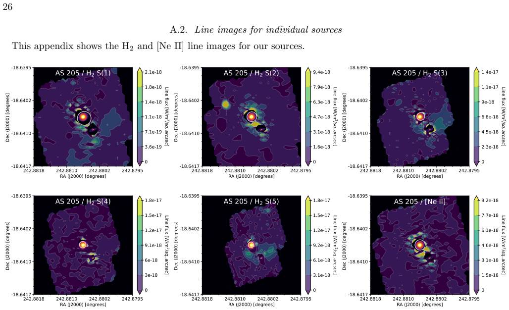
The winds appears to originate primarily from the northern component, AS 205N
AS 205 shows prominent and spatially extended H 2 emission, particularly in the strong ortho H2 lines, consistent with a wide-angle wind. The winds appears to originate primarily from the northern component, AS 205N. Given the close separation of the two components, the wind may also interact with the secondary star, potentially influencing the observed s...
-
[2]
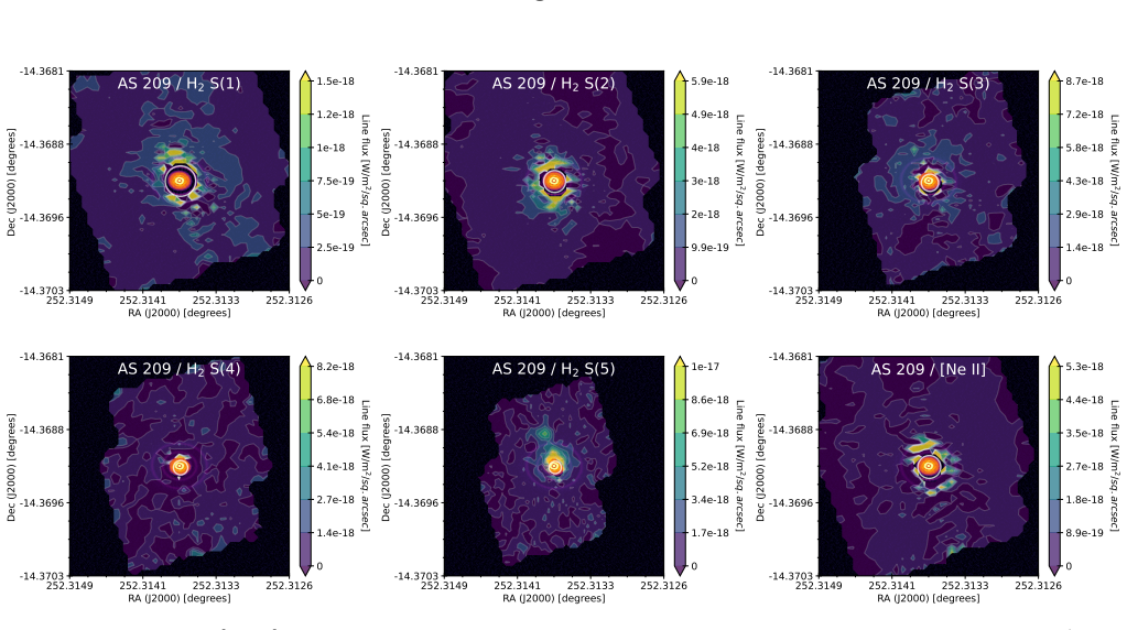
AS 209 is a moderately inclined disk. The observed H 2 morphology is consistent with this viewing geometry, with emission symmetric around the central source. Residual features associated with PSF subtraction are present in the immediate vicinity of the central source, but the extended emission beyond this region remains clearly detectable mainly in S(1),...
-
[3]
CI Tau exhibits a clear wide-angle wind. Only the blue-shifted side of the wind is detected, likely because the red-shifted emission is obscured by the disk. The wind is detected in the S(1), S(2), S(3), and S(5) lines. The S(4) line is faint and is dominated by PSF artifacts close to the center. The monopolar wind shows has a large opening angle. Complem...
-
[4]
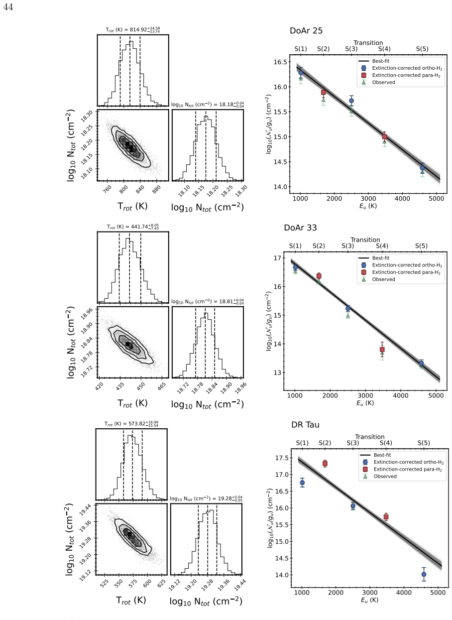
DoAr 25 stands out in the sample because its dust disk is observed in absorption against bright background H 2 emission, particularly in the S(1), S(2), and S(3) lines. The uniform background line emission originates from the photon-dominated region (PDR) near the Ophiuchus core. Superimposed on the background emission, the H2 data show clear signatures o...
-
[5]
We detect extended H 2 emission associated with the source in the S(1), S(2), and S(3) lines
DoAr 33 shows strong, uniform background H 2 emission in the S(1) and S(2) lines. We detect extended H 2 emission associated with the source in the S(1), S(2), and S(3) lines. The S(4) line shows little to no evidence of wind-like emission, while the S(5) line is affected by residal instrumental artifacts and PSF subtraction effects, making detailed inter...
-
[6]
This is consistent with the face-on orientation of the system
DR Tau is a nearly face-on disk, which exhibits faint extended H2 emission, and a symmetric morphology around the central source. This is consistent with the face-on orientation of the system. However, the faint nature of the extended component and limited S/N prevents further characterization of the spatial structure of the emission
-
[7]
Elias 20 is superimposed on bright background H 2 line emission associated with the the Ophiuchus core PDR. The background H 2 emission exhibits a gradient that increases toward the northeast, reflecting the structured nature of the PDR environment. The source displays a monopolar outflow, particularly prominent in the higher-J transitions (S(3)–S(5)), wh...
-
[8]
Elias 24 shows a ring-like morphology with a bright knot to the northeast in all H 2 lines. The ring is asymmetric, extending more along the northeast–southwest direction and less along the east–west direction. The bright northeastern knot stands out as a localized enhancement in H2 emission, suggesting a region of higher excitation, density, or possible ...
-
[9]
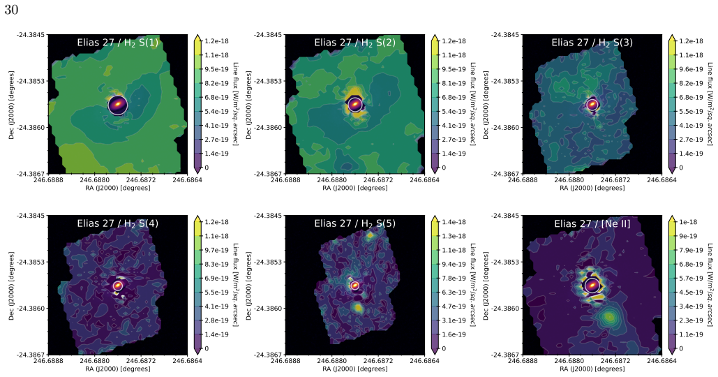
Elias 27 is observed in silhouette against strong background H 2 line emission from the Ophiuchus PDR in the S(1) and S(2) lines due to the dust in the disk. In the S(3) and S(5) lines, a monopolar outflow extending from the disk along the northeast side is observed. Extended [Ne II] emission is observed, indicating the presence of a collimated, ionized j...
-
[10]
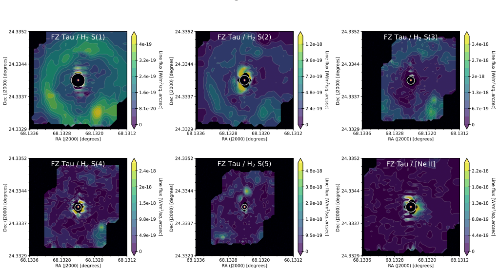
FZ Tau is a moderately inclined system. It represents one of the clearest examples of ring-like H 2 emission in our sample, with an average radius of∼2.4 ′′ (310 au) and a width of about 1.15 ′′ (148 au) (Pontoppidan et al. 2024b). A localized region of enhanced emission is visible toward the southwest portion of the ring, suggesting possible asymmetry in...
-
[11]
The emission is diffuse, without a clear preferred orientation
GK Tau shows extended H 2 emission in the S(1), S(2), S(3), and S(5) lines. The emission is diffuse, without a clear preferred orientation. There are no obvious morphological signatures indicative of a collimated wind. The lack of structure suggests that any molecular wind, if present, is intrinsically weak with a wide opening angle
-
[12]
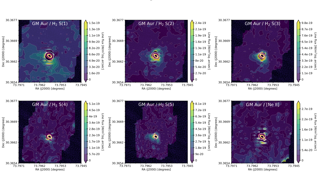
GM Aur exhibits a monopolar outflow oriented perpendicular to the dust disk plane detected in all observed H 2 lines. The emission traces a blue-shifted wide-angle structure extending away from the central source, consistent with a molecular wind emerging from the disk surface, while the red-shifted emission is obscured by the dust disk. GM Aur one of the...
-
[13]
GO Tau shows weak extended emission in the S(3), S(4), and S(5) lines. In contrast, the S(1) line reveals more discernible structure, suggestive of a wide-angle outflow and a disk silhouette with major axis oriented north-east/south-west
-
[14]
GQ Lup shows tentative extended emission with a wide-angle morphology in the S(1), S(2), and S(3) lines. Some PSF subtraction artifacts are present, particularly in the S(5) line, where a bright artifact is visible to the north of the source
-
[15]
The extended emission is concentrated around the star
GW Lup shows bright H 2 emission surrounding the central source in the S(1) and S(2) lines. The extended emission is concentrated around the star. Some of the bright features seen in the S(2) line near the central source may be caused by PSF subtraction artifacts
-
[16]
The apparent bright emission surrounding the star is consistent with PSF subtraction artifacts
HD 142666, HD 143006, HD 163296, and MWC 480 are Herbig Ae stars and show no extended H 2 emission in any of the observed lines. The apparent bright emission surrounding the star is consistent with PSF subtraction artifacts
-
[17]
HP Tau exhibits a striking ring-like H 2 morphology with a tail extending toward the west. The tail is prominent and coherent, suggesting material flowing or being entrained along this direction. In addition, the [Ne II] emission is also spatially extended along the western tail, indicating that both warm molecular and ionized gas trace the same outflow o...
-
[18]
HT Lup is a triple system with bright continuum emission. The primary component is associated with extended H2 emission, although not with an classical wind-like morphology. A tentative wide-angle wind component becomes more discernible in the S(3), S(4), and S(5) lines. This suggests that the primary hosts a molecular wind that is partially disrupted by ...
-
[19]
The northwestern lobe of the outflow has lower S/N in lines higher than S(1) and S(2)
IQ Tau is an inclined source that exhibits a clear bipolar H 2 outflow oriented perpendicular to the dust disk plane. The northwestern lobe of the outflow has lower S/N in lines higher than S(1) and S(2). The [Ne II] emission appears slightly extended along the outflow direction, suggesting that both warm molecular and ionized gas trace the outflow structure. 25
-
[20]
The bipolar structure is well-defined across the observed H 2 lines
IRAS 04385+2550 is moderately inclined (i= 60 ◦) and presents an unambiguous example of wide-angle bipolar H2 emission, reminiscent of emission seen in protostars, though with a significantly wider opening angle. The bipolar structure is well-defined across the observed H 2 lines. This demonstrates that bipolar winds can be visible even in sources that ar...
-
[21]
The higher-Jtransitions have lower S/N
MY Lup exhibits a clear bipolar morphology in the H 2 S(1) line, with tentative evidence for the S(2) line. The higher-Jtransitions have lower S/N. Weak bipolar emission is detected in the S(3) line, while the S(4) line shows little to no detectable emission. The [Ne II] emission is marginally extended
-
[22]
The symmetric structure is consistent with the nearly face-on orientation of this system
RU Lup shows bright, but compact, emission close to the central source in the S(1), S(2), and S(3) transitions, suggesting that any extended molecular wind is confined to small spatial scales. The symmetric structure is consistent with the nearly face-on orientation of this system
-
[23]
RY Lup is unique within the sample, exhibiting H 2 emission both parallel and perpendicular to the disk plane. The perpendicular component likely traces a molecular outflow or wind emerging from the disk surface, whereas the emission aligned with the disk may originate from cooler, quiescent disk gas. This dual morphology provides a rare view of both the ...
-
[24]
SR 4 is dominated by bright background H 2 emission originating from a nearby PDR in the Ophiuchus core, showing a clear spatial gradient increasing from the southwestern to the northeastern side. No definitive sig- natures of outflows or winds are detected in the H 2 emission, except in the S(5) transition. Extended [Ne II] emission is centered on the so...
-
[25]
SY Cha exhibits a conical monopolar H 2 outflow detected in all observed transitions, oriented toward the east (Schwarz et al. 2025a). Emission from the western side is observed, albeit significantly weaker. Additionally, SY Cha shows an extended [Ne II] jet on both sides of the disk, aligned along the wide-angle H 2 wind, indicating the presence of ioniz...
-
[26]
Sz 114 is a nearly face-on source (i= 20 ◦). The extended emission is concentrated around the central source, consistent with a face-on disk wind, and is detected in all observed H 2 lines
-
[27]
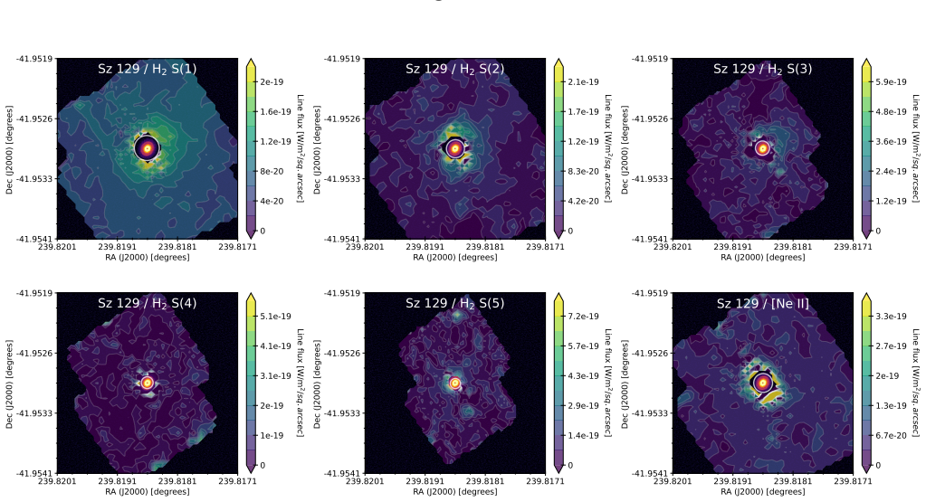
Sz 129 is a low-inclination source (i= 34 ◦). Extended emission from S(1), S(2), and S(3) H 2 lines is concentrated around the central source, consistent with a face-on disk wind. The [Ne II] emission is also marginally extended
-
[28]
The [Ne II] emission also appears extended, albeit more compact
TW Cha displays a centrally concentrated emission from the S(1), S(2), S(3), and S(5) lines, distributed sym- metrically around the central source, consistent with a face-on disk wind. The [Ne II] emission also appears extended, albeit more compact
-
[29]
The emission appears symmetric around the central source and likely traces the wide-angle disk wind
TW Hya shows a clear, symmetric, extended H2 morphology in all observed lines, consistent with a nearly face-on disk wind. The emission appears symmetric around the central source and likely traces the wide-angle disk wind. The [Ne II] emission also appears extended, albeit more compact
-
[30]
The bubble has a brighter rim and in the inner region is less bright
VZ Cha exhibits an unusual H 2 outflow morphology characterized by a bubble-like structure on the northwestern side of the source. The bubble has a brighter rim and in the inner region is less bright. The bubble component appears offset from the central source, possibly indicating a past episodic ejection event. The [Ne II] emission clearly reveals a jet ...
-
[31]
WSB 52 exhibits a wide-angle H 2 outflow. The S(1) transition is dominated by bright, extended emission, while the higher-excitation H 2 lines reveal a weaker but discernible bipolar morphology. The southwestern side of the outflow appears brighter than the northeastern side, indicating asymmetry in the emission or excitation conditions. The source also s...
discussion (0)
Sign in with ORCID, Apple, or X to comment. Anyone can read and Pith papers without signing in.