arxiv: 2605.07596 · v2 · submitted 2026-05-08 · 📊 stat.ML · cs.LG

Recognition: no theorem link

A Refined Generalization Analysis for Extreme Multi-class Supervised Contrastive Representation Learning

Antoine Ledent, Nong Minh Hieu

Pith reviewed 2026-05-12 03:25 UTC · model grok-4.3

classification 📊 stat.ML cs.LG

keywords contrastive representation learninggeneralization boundssample complexitymulti-class classificationU-statisticslong-tailed distributionssupervised learningextreme classification

0 comments

The pith

A new cross-class risk estimator for supervised contrastive learning produces generalization bounds whose sample complexity scales with the number of classes rather than the frequency of the rarest class.

A machine-rendered reading of the paper's core claim, the machinery that carries it, and where it could break.

The paper works to tighten the theoretical sample requirements for learning representations via supervised contrastive methods when the number of classes is large and their frequencies are uneven. It replaces the previous per-class uniform concentration requirement with a single estimator that tracks how risk behaves across the whole collection of classes, allowing the derived excess-risk bound to depend only on the total number of classes R instead of the inverse square root of the smallest class probability. This matters for data sets that contain many infrequent classes, because those classes add little to the overall population risk yet previously dictated much larger training sets. A reader following the argument would see that the new estimator, built from U-statistics on tuples drawn from a finite labeled pool, removes an artificial dependence on the tail and yields an O(k) sample complexity under mild conditions on the class frequencies, where k counts the samples per contrastive tuple.

Core claim

We improve upon the previous work and prove a bound with a sample complexity of the same order as the number of classes R, regardless of the distribution over classes. Furthermore, we formulate a different estimator that captures the concentration of the risk across classes, enabling sharper bounds in extreme multi-class learning scenarios, especially where class distributions are long-tailed. Under mild assumptions on the class distributions, the resulting sample complexity is O(k) where k is the number of samples per tuple.

What carries the argument

The cross-class risk estimator constructed via U-statistics on dependent tuples, which aggregates risk concentration information over the entire set of classes instead of demanding uniform concentration inside each individual class.

If this is right

Excess risk bounds become independent of the probability of the rarest class.
The number of required training tuples grows linearly with the total number of classes even when many tail classes are present.
Sharper generalization guarantees hold specifically for the long-tailed regimes typical of extreme multi-class problems.
U-statistic analysis now applies to contrastive tuple sampling without the previous uniform-per-class restriction.

Where Pith is reading between the lines

These are editorial extensions of the paper, not claims the author makes directly.

The result suggests that data collection efforts can focus on covering all classes rather than oversampling rare ones to meet theoretical guarantees.
Similar cross-class aggregation techniques might tighten bounds for other tuple-based losses that suffer from dependence induced by finite labeled pools.
Direct empirical measurement of risk concentration across classes on real data sets could confirm the predicted improvement over per-class analyses.

Load-bearing premise

Mild conditions on the class probability distribution hold so that overall risk concentrates across classes without requiring the same concentration inside every single class.

What would settle it

Collect a long-tailed labeled data set with known class frequencies, train the contrastive model with increasing numbers of tuples per class, and check whether the measured excess risk decreases proportionally to the number of tuples per class rather than stalling at a level governed by the rarest class frequency.

Figures

Figures reproduced from arXiv: 2605.07596 by Antoine Ledent, Nong Minh Hieu.

**Figure 1.** Figure 1: Synthetic data experiment results for representation learning on an imbalanced dataset. Left: PCA reduced representations of the model trained with sub-sampled estimation of UN as empirical risk. Right: PCA reduced representations of model trained with sub-sampled estimation of U hl N as empirical risk. Both plots show representations of 100 data points from top five rarest classes in the synthesized datas… view at source ↗

**Figure 2.** Figure 2: Final contrastive test loss for the model trained using subsampled estimations of two U-Statistics formulations, UN (blue) and U hl N , as empirical risks (red) on synthetic dataset. Example 4.1 (Typical Extreme Scenario). Suppose that ρr ⩽ 1 k+1 for all r ∈ [R]. Then, for triplet learning (k = 1), we have 1 − τ = 1 − PR r=1 ρ 2 r ⩾ 1 − 1 2 PR r=1 ρr = 1 2 . On the other hand, for k ⩾ 2, we have: 1 − τ = … view at source ↗

**Figure 3.** Figure 3: Comparison of the tuple selection process for each permutation of the labeled dataset S. For simplicity, only two classes are considered in this illustration (green and red). Left: Construction of the estimator U hl N from Hieu & Ledent (2025): Tuples are selected class-wise for each component estimator defined in Hieu & Ledent (2025). U hl N is expressed as an average of this construction over all permuta… view at source ↗

**Figure 4.** Figure 4: Class distributions used for synthetic (left) and real (right) data experiments. For the real data experiments, we used the same class distribution structure as depicted in the figure above to create subsets from all real datasets (MNIST, FashionMNIST and CIFAR10). Remark I.1. From Algorithm 2, there is an interesting effect of the chosen sub-sampling distribution q in Eqn. (105) on how the sub-sampled est… view at source ↗

read the original abstract

Contrastive Representation Learning (CRL) has achieved strong empirical success in multiple machine learning disciplines, yet its theoretical sample complexity remains poorly understood. Existing analyses usually assume that input tuples are identically and independently distributed, an assumption violated in most practical settings where contrastive tuples are constructed from a finite pool of labeled data, inducing dependencies among tuples. While one recent work analyzed this learning setting using U-Statistics to estimate the population risk, the techniques used therein require the risk of each class to concentrate uniformly, making excess risk bounds scale in the order of $\rho_{\min}^{-{1}/{2}}$ where $\rho_{\min}$ denotes the probability of the rarest class. Such a dependency can be overly pessimistic in the extreme multiclass settings where there are many tail classes which contribute minimally to the overall population risk. Our contributions are two-fold. Firstly, we improve upon the previous work and prove a bound with a sample complexity of the same order as the number of classes $R$, regardless of the distribution over classes. Furthermore, we formulate a different estimator that captures the concentration of the risk \textit{across classes}, enabling sharper bounds in extreme multi-class learning scenarios, especially where class distributions are long-tailed. Under mild assumptions on the class distributions, the resulting sample complexity is $\mathcal{{O}}(k)$ where $k$ is the number of samples per tuple.

Editorial analysis

A structured set of objections, weighed in public.

Desk editor's note, referee report, simulated authors' rebuttal, and a circularity audit. Tearing a paper down is the easy half of reading it; the pith above is the substance, this is the friction.

Desk Editor's Note private letter to a colleague

This paper tightens sample complexity for contrastive learning in long-tailed multi-class settings by replacing per-class concentration with a cross-class risk estimator.

read the letter

The punchline is that this paper refines the generalization bounds for supervised contrastive learning in long-tailed multi-class settings by using a cross-class risk concentration estimator, which removes the dependence on the probability of the rarest class. It improves on earlier U-statistic analyses by proving a sample complexity that scales with the number of classes R regardless of the distribution, and under mild assumptions, even with the number of samples per tuple k. The new estimator is the key novelty here, shifting focus from per-class to across-class risk to better suit extreme multi-class scenarios where many classes are rare but don't dominate the overall risk. The work does a good job identifying the dependency problem when constructing contrastive tuples from a finite pool of labeled data, which violates the usual i.i.d. assumption. Applying U-statistic theory to this setting is appropriate, and the idea to concentrate risk across classes rather than uniformly is a reasonable way to get tighter bounds in long-tailed distributions. The soft spots are around the mild assumptions needed for the O(k) bound. These aren't specified in the abstract, so it's unclear how restrictive they are in practice. If they hold only for certain distributions, the practical impact might be narrower than claimed. The soundness can't be fully assessed without the derivations, but the argument doesn't show obvious circularity or inconsistencies based on the summary. This is for people working on theoretical foundations of contrastive representation learning, especially in imbalanced data regimes. A reader interested in sample complexity for real-world multi-class problems would get something out of the new estimator concept. It deserves a serious referee because the problem it tackles is relevant and the proposed fix is coherent, even if the details require checking.

Referee Report

2 major / 1 minor

Summary. The manuscript claims to advance the theoretical analysis of supervised contrastive representation learning in extreme multi-class settings. It improves on prior U-statistic-based bounds by deriving excess risk guarantees whose sample complexity scales with the number of classes R independently of the minimum class probability rho_min, and introduces a new cross-class risk estimator whose concentration properties yield O(k) sample complexity (k = samples per tuple) under mild assumptions on the class distribution, with particular benefit for long-tailed regimes.

Significance. If the stated improvements hold, the work would meaningfully relax pessimistic dependencies on rare-class probabilities that appear in earlier analyses of dependent contrastive tuples. The shift from uniform per-class concentration to across-class concentration is a coherent technical move for handling imbalance, and the explicit use of U-statistics to account for finite-pool dependence is a strength. Such bounds could inform algorithm design and data-collection strategies in practical extreme multi-class contrastive learning.

major comments (2)

[Abstract] Abstract: the central claim of an O(R) sample-complexity bound independent of rho_min rests on the specific U-statistic estimator and concentration argument; without the explicit theorem statement, the definition of the estimator, and the key steps that remove the rho_min^{-1/2} factor, the improvement cannot be verified.
[Abstract] Abstract: the sharper O(k) bound is conditioned on 'mild assumptions on the class distributions' that enable the cross-class estimator; these assumptions are load-bearing for the long-tail claim and must be stated precisely (e.g., moment conditions, tail decay rates) together with a demonstration that they are satisfied by typical long-tailed distributions.

minor comments (1)

[Abstract] The abstract would be clearer if it briefly recalled the precise dependence on rho_min that appears in the cited prior work, allowing readers to quantify the stated improvement.

Simulated Author's Rebuttal

2 responses · 0 unresolved

We thank the referee for the careful reading and constructive comments on our manuscript. We address the major comments point by point below, providing clarifications from the full paper and indicating revisions made to improve verifiability and precision.

read point-by-point responses

Referee: [Abstract] Abstract: the central claim of an O(R) sample-complexity bound independent of rho_min rests on the specific U-statistic estimator and concentration argument; without the explicit theorem statement, the definition of the estimator, and the key steps that remove the rho_min^{-1/2} factor, the improvement cannot be verified.

Authors: The abstract is a concise summary, but the explicit theorem statements, estimator definitions, and concentration arguments are detailed in the body of the manuscript. Specifically, the U-statistic estimator is defined in Section 3.1, Theorem 3.1 states the O(R) excess risk bound independent of rho_min, and the proof in Section 3.2 shows how the variance bound is taken over the average class contribution rather than the minimum, removing the rho_min^{-1/2} factor. We have revised the abstract to include a direct reference to Theorem 3.1 and Section 3 for immediate verifiability. revision: yes
Referee: [Abstract] Abstract: the sharper O(k) bound is conditioned on 'mild assumptions on the class distributions' that enable the cross-class estimator; these assumptions are load-bearing for the long-tail claim and must be stated precisely (e.g., moment conditions, tail decay rates) together with a demonstration that they are satisfied by typical long-tailed distributions.

Authors: We agree that greater precision is needed for the assumptions supporting the O(k) bound. In the revised manuscript, Section 4.2 now explicitly states the required conditions: bounded fourth moments on the loss and polynomial tail decay with exponent greater than 1 on the class probabilities. A new Lemma 4.1 demonstrates that these hold for standard long-tailed distributions, including Zipf distributions with parameter alpha > 1, which are representative of extreme multi-class settings. This addition directly supports the long-tail applicability claim. revision: yes

Circularity Check

0 steps flagged

No significant circularity in derivation chain

full rationale

The paper derives its O(R) and O(k) sample complexity bounds from standard U-statistic concentration applied to a newly introduced cross-class risk estimator, under explicitly stated mild assumptions on class distributions. The abstract and summary show no reduction of the target bounds to fitted parameters, self-defined quantities, or load-bearing self-citations; the move from uniform per-class to across-class concentration is a direct consequence of the estimator definition and does not loop back to the claimed results. The dependence on finite labeled pools is handled transparently via U-statistics without circularity.

Axiom & Free-Parameter Ledger

0 free parameters · 1 axioms · 0 invented entities

The central claim rests on U-statistic theory for dependent samples plus mild assumptions on class distributions; no free parameters or invented entities are introduced in the abstract.

axioms (1)

domain assumption Mild assumptions on the class distributions
Invoked to obtain the O(k) sample complexity bound in long-tailed extreme multi-class settings.

pith-pipeline@v0.9.0 · 5547 in / 1198 out tokens · 75205 ms · 2026-05-12T03:25:42.100247+00:00 · methodology

Review history (2 revisions) →

discussion (0)

Reference graph

Works this paper leans on

49 extracted references · 49 canonical work pages

[1]

Awasthi, P., Dikkala, N., and Kamath, P

URL https://proceedings.mlr.press/ v151/ash22a.html. Awasthi, P., Dikkala, N., and Kamath, P. Do more negative samples necessarily hurt in contrastive learn- ing? In Chaudhuri, K., Jegelka, S., Song, L., Szepesvari, C., Niu, G., and Sabato, S. (eds.),Pro- ceedings of the 39th International Conference on Ma- chine Learning, volume 162 ofProceedings of Mach...

work page
[2]

Bao, H., Nagano, Y ., and Nozawa, K

URL https://proceedings.mlr.press/ v162/awasthi22b.html. Bao, H., Nagano, Y ., and Nozawa, K. On the surrogate gap between contrastive and supervised losses. InInterna- tional Conference on Machine Learning, pp. 1585–1606. PMLR, 2022. Bartlett, P. L., Foster, D. J., and Telgarsky, M. Spectrally- normalized margin bounds for neural networks. InAd- vances i...

work page 2022
[3]

ISBN 9781713829546

Curran Associates Inc. ISBN 9781713829546. Chen, T., Kornblith, S., Norouz, M., and Hinton, G. A simple framework for contrastive learning of visual rep- resentations. InInternational Conference on Machine Learning, 2020. Chen, T.-S., Hung, W.-C., Tseng, H.-Y ., Chien, S.-Y ., and Yang, M.-H. Incremental false negative detection for con- trastive learning...

work page arXiv 2020
[4]

natural estimator

Springer International Publishing. ISBN 978-3- 319-46379-7. McDiarmid, C.On the method of bounded differences, pp. 148–188. London Mathematical Society Lecture Note Series. Cambridge University Press, 1989. Nozawa, K. and Sato, I. Understanding negative samples in instance discriminative self-supervised representation learning. InAdvances in Neural Inform...

work page 1989
[5]

Both ¯UΩ(f)and ¯UΛ(f)are asymptotically unbiased estimators ofL Ω(f)andL Λ(f)

work page
[6]

RX r=1 ωπ r UΩπr (f) # =E

They are different fromU Ω(f)andU Λ(f)by negligible factors. Prior to presenting the proof for Proposition D.6, we first start by proving the asymptotic unbiasedness of ¯UΩ(f) and ¯UΛ(f). Before that, for completeness of definitions, we define the class-wise risksL r Ω andL r Λ as follows: Lr Ω(f) =E X,X+∼D⊗2 r {X − i } k i=1∼ ¯D⊗k h ℓϕ,f X, X+, X − i k i...

work page
[7]

redundant

We start with a bag of N balls with M special balls and we mark two random special balls as “redundant”. Next, we drawk+ 2balls without replacement from theNballs

work page
[8]

To sampleX, we take the firstkballs in the previously selectedk+ 2balls

work page
[9]

redundant

To sampleY, we follow the following procedure: • If the firstkballs did not contain the “redundant” ones, it is also a valid draw ofY. • If one “redundant” showed up in the firstk draws, replace that with one of the last two balls (note that there must be one non-redundant balls among the last two). • If two “redundant showed up in the firstkdraws, replac...

work page
[10]

42 Refined Generalization Analysis for SCRL Proof.LetΦ :R R →[0,1]be defined as follows: Φ(q1,

ln(R+ 1)/∆ N # ,(77) with probability of at least1−∆where∥ρ∥ 2 2 =PR r=1 ρ2 r. 42 Refined Generalization Analysis for SCRL Proof.LetΦ :R R →[0,1]be defined as follows: Φ(q1, . . . , qR) = 1− RX r=1 qr [1−q r]k . Then, we have: |τ−bτ|=|Φ(ρ 1, . . . , ρR)−Φ(bρ1, . . . ,bρR)| ⩽max {qr}R r=1∈∆R ∥∇Φ(q1, . . . , qR)∥2 · ∥u−E[u]∥ 2, where u={bρ 1, . . . ,bρR} ∈∆...

work page
[11]

Solving the above quadratic equation yields: λ= 2 ln(R+1)/∆ 3 + q 4 ln2(R+1)/∆ 9 + 8N(1− ∥ρ∥ 2

ln R+ 1 ∆ = 0. Solving the above quadratic equation yields: λ= 2 ln(R+1)/∆ 3 + q 4 ln2(R+1)/∆ 9 + 8N(1− ∥ρ∥ 2

work page
[12]

ln R+1 ∆ 2N = ln(R+ 1)/∆ 3N + 1 N s ln2(R+ 1)/∆ 9 + 2N(1− ∥ρ∥ 2

work page
[13]

In other words, we have: ∥u−ρ∥ 2 ⩽ ln(R+ 1)/∆ 3N + 1 N s ln2(R+ 1)/∆ 9 + 2N(1− ∥ρ∥ 2

ln R+ 1 ∆ . In other words, we have: ∥u−ρ∥ 2 ⩽ ln(R+ 1)/∆ 3N + 1 N s ln2(R+ 1)/∆ 9 + 2N(1− ∥ρ∥ 2

work page
[14]

ln R+ 1 ∆ ⩽ ln(R+ 1)/∆ 3N + 1 N " ln(R+ 1)/∆ 3 + r 2N(1− ∥ρ∥ 2

work page
[15]

ln R+ 1 ∆ # = 2 ln(R+ 1)/∆ 3N + r 2(1− ∥ρ∥ 2

work page
[16]

Combine this with the bound on∥∇Φ(q 1,

ln(R+ 1)/∆ N , 44 Refined Generalization Analysis for SCRL with probability of1−∆. Combine this with the bound on∥∇Φ(q 1, . . . , qR)∥2, we have: |τ−bτ|⩽ |R−(k+ 1)|√ R 1− 1 R k−1 · ∥u−ρ∥ 2 ⩽ |R−(k+ 1)|√ R 1− 1 R k−1" 2 ln(R+ 1)/∆ 3N + r 2(1− ∥ρ∥ 2

work page
[17]

well-behaved

ln(R+ 1)/∆ N # , with probability of at least1−∆, as desired. Proposition F.2(Multiplicative Concentration of 1−bτ).Let τ be the collision probability defined in Eqn. (12) andbτbe the plug-in estimator in Eqn.(76). For any∆∈(0,1), with probability of at least1−∆: 1−bτ⩾ C 2 1 + 1−γ 4k γ4k ¯C −1 (1−τ)as long asN⩾8γ −1 4k ln 2 ∆ + 12kln 2R ∆ ,(79) 1−τ⩾ C 2 1...

work page
[18]

1 2k + 1− 1 4k2 k# . When k= 1 then we have ρmax(1−ρ max)k =ρ max(1−ρ max)⩽1−ρ max. Therefore, for any value of k⩾1 , we have the following general upper bound: 1−τ 2 ⩽(1−ρ max)

Otherwise, we have Γ∪ ¯Γ∗ = [R]\ {r ∗} wherer ∗ = arg maxr∈[R] ρr. Claim (i): For any δ∈(0,1) , as long as we have N⩾32k 2 ln R δ , then (1−bρr)k ⩾ 1√ 2(1−ρ r)k with probability of at least1−δfor allr∈ ¯Γ∗. For allr∈[R]such thatρ r ⩽ 1 2, we have: P [1−bρr]k ⩽ [1−ρ r]k √ 2 =P [1−bρr]k ⩽ h 2− 1 2k (1−ρ r) ik =P 1−bρr ⩽2 − 1 2k (1−ρ r) ⩽exp −1 2 1− 1 2 1 2k...

work page 2016
[19]

ln 6(R+1) ∆ N   , with probability of at least 1−∆ as long as N⩾3γ −1 2k ln 12 ∆ + 16kln 12R ∆ where the constants C, ¯C, γ2k,bγ4k are defined in Proposition F .2 andΨ(R, k) = |R−(k+1)|√ R 1− 1 R k−1 . Furthermore, when R⩾k , as long as we have N⩾k×max n 3γ−1 2k ln(12/∆) k + 16 ln(12R/∆), R o , we have: sup f∈F ¯UN(f)−L ϕ(f) ⩽O " CN(H) 1−bτ r k N + B ...

work page
[20]

6R n−R + 8R 3N ln 4R/δ+ r 8(R−1) ln 4R/δ 3N + 8 r ln 2/δ n−R #) + BΨ(R, k) (1−τ)(1−bτ)

lnR/∆ N # ,(90) with probability of at least1−∆. 53 Refined Generalization Analysis for SCRL Proof.We have: sup f∈F ¯UN(f)−L ϕ(f) = sup f∈F 1 1−bτ ¯UΩ(f)− bτ 1−bτ ¯UΛ(f)− 1 1−τ LΩ(f) + τ 1−τ LΛ(f) ⩽sup f∈F 1 1−bτ ¯UΩ(f)− 1 1−τ LΩ(f) | {z } α + sup f∈F bτ 1−bτ ¯UΛ(f)− τ 1−τ LΛ(f) | {z } β . Now, we proceed to bound theαandβterms. Firstly, we have: α⩽ 1 1−b...

work page
[21]

6R n−R + 8R 3N ln 4R/δ+ r 8(R−1) ln 4R/δ 3N + 8 r ln 2/δ n−R #) + 2BΨ(R, k) C(1−bτ)2 1 + 1−bγ4k bγ4k ¯C

ln(R+ 1)/δ N # , with probability of at least 1−2δ (union bound) and Ψ(R, k) = |R−(k+1)|√ R 1− 1 R k−1 . Furthermore, by Proposition F.2 (relative error of bτ), we have 1−τ⩾ C 2 h 1 + 1−bγ4k bγ4k ¯C i−1 (1−bτ), with probability of at least 1−δ as long as N⩾3γ −1 2k ln 2 δ + 16kln 2R ∆ . As a result: α⩽ 1 1−bτ ( 2Rµ∗(H) +B " 6R n−R + 8R 3N ln 4R/δ+ r 8(R−1...

work page
[22]

12R m−2R + 8R 3N ln 4R/δ+ r 8(R−1) ln 4R/δ 3N + 8 r ln 2/δ m−2R #) + 2BΨ(R, k) C(1−bτ)2 1 + 1−bγ4k bγ4k ¯C

ln(R+ 1)/δ N # , with probability of at least 1−3δ (by union bound) as long as N⩾3γ −1 2k ln 2 δ + 16kln 2R δ . Similarly, we can bound β using the concentration result of ¯UΛ(f)in Theorem E.11 and Proposition F.1, Proposition F.2. Specifically, we have: β⩽ bτ 1−bτ sup f∈F ¯UΛ(f)−L Λ(f) + B|bτ−τ| (1−τ)(1−bτ) ⩽ bτ 1−bτ ( 2Rν∗(H) +B " 12R m−2R + 8R 3N ln 4R...

work page
[23]

12R m−2R + 8R 3N ln 4R/δ+ r 8(R−1) ln 4R/δ 3N + 8 r ln 2/δ m−2R # (bτ⩽1) + 2BΨ(R, k) C(1−bτ)2 1 + 1−bγ4k bγ4k ¯C

ln(R+ 1)/δ N # ⩽ 2bτRν∗(H) 1−bτ + B 1−bτ " 12R m−2R + 8R 3N ln 4R/δ+ r 8(R−1) ln 4R/δ 3N + 8 r ln 2/δ m−2R # (bτ⩽1) + 2BΨ(R, k) C(1−bτ)2 1 + 1−bγ4k bγ4k ¯C " 2 ln(R+ 1)/δ 3N + r 2(1− ∥ρ∥ 2

work page
[24]

r ln 2/δ n−R + r ln 2/δ m−2R # + 2B 1−bτ

ln(R+ 1)/δ N # , 54 Refined Generalization Analysis for SCRL with probability of at least 1−3δ as long as N⩾3γ −1 2k ln 2 δ + 16kln 2R δ . Combining the bounds of α and β, we have: sup f∈F ¯UN(f)−L ϕ(f) ⩽ 2Rµ∗(H) + 2bτRν∗(H) 1−bτ + 8B 1−bτ "r ln 2/δ n−R + r ln 2/δ m−2R # + 2B 1−bτ " 3R n−R + 6R m−2R + 8R 3N ln 4R/δ+ r 8(R−1) ln 4R/δ 3N # + 4BΨ(R, k) C(1−b...

work page
[25]

Rµ∗(H) +bτRν∗(H) 1−bτ + B 1−bτ

ln(R+ 1)/δ N # ⩽O " Rµ∗(H) +bτRν∗(H) 1−bτ + B 1−bτ "r ln 1/δ n−R + r ln 1/δ m−R # + BΨ(R, k) (1−bτ)2 1 + 1−bγ4k bγ4k r (1− ∥ρ∥ 2

work page
[26]

CN(H) r k N # ,R ν∗(H)⩽O

lnR/δ N # , with probability of at least 1−6δ as long as N⩾3γ −1 2k ln 2 δ + 16kln 2R δ . Setting δ= ∆/6 yields the desired complete bound. Furthermore, as long asN⩾2Rk, we have: r 1 n−R = s 1 2⌊ N k ⌋ −R ⩽ s 1 N/k−R ⩽ r k N−Rk ∈ O r k N ! . Similarly, we also have 1√m−2R ⩽O q k N . Therefore, as long as N⩾k×max n 3γ−1 2k ln(12/∆) k + 16 ln(12R/∆), R o (s...

work page
[27]

lnR/∆ N # ⩽O " CN(H) 1−bτ r k N + B √ R (1−bτ)2 1 + 1−bγ4k bγ4k r (1− ∥ρ∥ 2

work page
[28]

In the last inequality, we haveΨ(R, k)∈ O( √ R)given thatR⩾k

lnR/∆ N # , with probability of at least1−∆, as desired. In the last inequality, we haveΨ(R, k)∈ O( √ R)given thatR⩾k. Theorem G.4(cf. Table 1).Let F be a class of representation functions and let ¯UN(f) be defined for each f∈ F in Eqn.(16). Then, for any∆∈(0,1), we have: sup f∈F ¯UN(f)−L ϕ(f) ⩽ 2Rµ∗(H) + 2τRν∗(H) 1−τ + 8B 1−τ "r ln 12/∆ n−R + r ln 12/∆ m...

work page
[29]

ln 6(R+1) ∆ N   , 55 Refined Generalization Analysis for SCRL with probability of at least 1−∆ as long as N⩾8γ −1 4k ln 12 ∆ + 12kln 12R ∆ where the constants C, ¯C, γ2k, γ4k are defined in Proposition F .2 andΨ(R, k) = |R−(k+1)|√ R 1− 1 R k−1 . Furthermore, when R⩾k , as long as we have N⩾k×max n 8γ−1 4k ln(12/∆) k + 12 ln(12R/∆), R o , we have: sup ...

work page
[30]

6R n−R + 8R 3N ln 4R/δ+ r 8(R−1) ln 4R/δ 3N + 8 r ln 2/δ n−R #) + BΨ(R, k) (1−τ)(1−bτ)

lnR/∆ N # ,(92) with probability of at least1−∆. Proof.Similar to Theorem G.3, we have: sup f∈F ¯UN(f)−L ϕ(f) ⩽sup f∈F 1 1−bτ ¯UΩ(f)− 1 1−τ LΩ(f) | {z } α + sup f∈F bτ 1−bτ ¯UΛ(f)− τ 1−τ LΛ(f) | {z } β . Bounding theαterm, we have: α⩽ 1 1−τ sup f∈F ¯UΩ(f)−L Ω(f) + sup f∈F | ¯UΩ(f)| · 1 1−bτ − 1 1−τ ⩽ 1 1−τ sup f∈F ¯UΩ(f)−L Ω(f) + B|bτ−τ| (1−τ)(1−bτ) . The...

work page
[31]

6R n−R + 8R 3N ln 4R/δ+ r 8(R−1) ln 4R/δ 3N + 8 r ln 2/δ n−R #) + 2BΨ(R, k) C(1−τ) 2 1 + 1−γ 4k γ4k ¯C

ln(R+ 1)/δ N # , with probability of at least 1−2δ (union bound) and Ψ(R, k) = |R−(k+1)|√ R 1− 1 R k−1 . Furthermore, by Proposition F.2 (relative error of bτ), we have 1−bτ⩾ C 2 h 1 + 1−γ4k γ4k ¯C i−1 (1−τ) with probability of at least 1−δ as long as N⩾8γ −1 4k ln 2 δ + 12kln 2R δ . Therefore: α⩽ 1 1−τ ( 2Rµ∗(H) +B " 6R n−R + 8R 3N ln 4R/δ+ r 8(R−1) ln 4...

work page
[32]

12R m−2R + 8R 3N ln 4R/δ+ r 8(R−1) ln 4R/δ 3N + 8 r ln 2/δ m−2R #) + 2BΨ(R, k) C(1−τ) 2 1 + 1−γ 4k γ4k ¯C

ln(R+ 1)/δ N # , with probability of at least1−3δ(by union bound) as long asN⩾8γ −1 4k ln 2 δ + 12kln 2R δ . Similarly, we have: β⩽ τ 1−τ ( 2Rν∗(H) +B " 12R m−2R + 8R 3N ln 4R/δ+ r 8(R−1) ln 4R/δ 3N + 8 r ln 2/δ m−2R #) + 2BΨ(R, k) C(1−τ) 2 1 + 1−γ 4k γ4k ¯C " 2 ln(R+ 1)/δ 3N + r 2(1− ∥ρ∥ 2

work page
[33]

12R m−2R + 8R 3N ln 4R/δ+ r 8(R−1) ln 4R/δ 3N + 8 r ln 2/δ m−2R # (τ⩽1) + 2BΨ(R, k) C(1−τ) 2 1 + 1−γ 4k γ4k ¯C

ln(R+ 1)/δ N # ⩽ 2τR ν∗(H) 1−τ + B 1−τ " 12R m−2R + 8R 3N ln 4R/δ+ r 8(R−1) ln 4R/δ 3N + 8 r ln 2/δ m−2R # (τ⩽1) + 2BΨ(R, k) C(1−τ) 2 1 + 1−γ 4k γ4k ¯C " 2 ln(R+ 1)/δ 3N + r 2(1− ∥ρ∥ 2

work page
[34]

r ln 2/δ n−R + r ln 2/δ m−2R # + 2B 1−τ

ln(R+ 1)/δ N # , 56 Refined Generalization Analysis for SCRL with probability of at least 1−3δ as long as N⩾8γ −1 4k ln 2 δ + 12kln 2R δ . Combining the bounds on α, β via the union bound, we have: sup f∈F ¯UN(f)−L ϕ(f) ⩽ 2Rµ∗(H) + 2τRν∗(H) 1−τ + 8B 1−τ "r ln 2/δ n−R + r ln 2/δ m−2R # + 2B 1−τ " 3R n−R + 6R m−2R + 8R 3N ln 4R/δ+ r 8(R−1) ln 4R/δ 3N # + 4B...

work page
[35]

Rµ∗(H) +τR ν∗(H) 1−τ + B 1−τ

ln(R+ 1)/δ N # ⩽O " Rµ∗(H) +τR ν∗(H) 1−τ + B 1−τ "r ln 1/δ n−R + r ln 1/δ m−R # + BΨ(R, k) (1−τ) 2 1 + 1−γ 4k γ4k r (1− ∥ρ∥ 2

work page
[36]

Setting δ= ∆/6 yields the desired complete bound

lnR/δ N # , with probability of at least 1−6δ as long as N⩾8γ −1 4k ln 2 δ + 12kln 2R δ . Setting δ= ∆/6 yields the desired complete bound. Applying the same arguments to obtain O-notation bound in Theorem G.3: When R⩾k , as long as N⩾k×max n 8γ−1 4k ln(12/∆) k + 12 ln(12R/∆), R o , we have: sup f∈F | ¯UN(f)−L ϕ(f)|⩽O " CN(H) 1−τ r k N + B √ R (1−τ) 2 1 +...

work page
[37]

Theorem G.5(cf

lnR/∆ N # , with probability of at least1−∆. Theorem G.5(cf. Theorem 4.5, Table 1).Let F be a class of representation functions and let ¯UN(f) be defined for each f∈ Fin Eqn.(16). Then, for any∆∈(0,1), we have: sup f∈F ¯UN(f)−L ϕ(f) ⩽ 2Rµ∗(H) + 2τRν∗(H) 1−τ + 8B 1−τ "r ln 12/∆ n−R + r ln 12/∆ m−2R # + 2B 1−τ   3R n−R + 6R m−2R + 8R 3N ln 24R ∆ + s 8(R−1...

work page
[38]

Furthermore, whenR⩾k, as long asN⩾k×max 164kln 24R ∆ + 100 ln( 12 ∆ ) k(1−τ) , R , we have: sup f∈F | ¯UN(f)−L ϕ(f)|⩽O " CN(H) 1−τ r k N + B √ R (1−τ) 2 r (1− ∥ρ∥ 2

ln 6(R+1) ∆ N   , with probability of at least 1−∆ as long as N⩾164k 2 ln 24R ∆ + 100 ln( 12 ∆ ) 1−τ where Ψ(R, k) = |R−(k+1)|√ R 1− 1 R k−1 . Furthermore, whenR⩾k, as long asN⩾k×max 164kln 24R ∆ + 100 ln( 12 ∆ ) k(1−τ) , R , we have: sup f∈F | ¯UN(f)−L ϕ(f)|⩽O " CN(H) 1−τ r k N + B √ R (1−τ) 2 r (1− ∥ρ∥ 2

work page
[39]

6R n−R + 8R 3N ln 4R/δ+ r 8(R−1) ln 4R/δ 3N + 8 r ln 2/δ n−R #) + BΨ(R, k) (1−τ)(1−bτ)

lnR/∆ N # , with probability of at least1−∆. Proof. Let δ∈(0,1) . Suppose that the minimum sample complexity N⩾164k 2 ln 4R δ + 100 ln( 2 δ) 1−τ is satisfied. Let us reuse the quantitiesα, βas defined in Theorem G.4: α= sup f∈F 1 1−bτ ¯UΩ(f)− 1 1−τ LΩ(f) , β= sup f∈F bτ 1−bτ ¯UΛ(f)− τ 1−τ LΛ(f) . 57 Refined Generalization Analysis for SCRL Combine Proposi...

work page
[40]

6R n−R + 8R 3N ln 4R/δ+ r 8(R−1) ln 4R/δ 3N + 8 r ln 2/δ n−R #) + 8BΨ(R, k) (1−τ) 2

ln(R+ 1)/δ N # ⩽ 1 1−τ ( 2Rµ∗(H) +B " 6R n−R + 8R 3N ln 4R/δ+ r 8(R−1) ln 4R/δ 3N + 8 r ln 2/δ n−R #) + 8BΨ(R, k) (1−τ) 2 " 2 ln(R+ 1)/δ 3N + r 2(1− ∥ρ∥ 2

work page
[41]

12R m−2R + 8R 3N ln 4R/δ+ r 8(R−1) ln 4R/δ 3N + 8 r ln 2/δ m−2R #) + 8BΨ(R, k) (1−τ) 2

ln(R+ 1)/δ N # , with probability of at least 1−3δ . Similarly, combining Proposition F.1 (absolute error of bτ), Proposition F.7 (generic multiplicative error ofbτ) and Theorem E.11 (absolute error of ¯UΛ(f)) via union bound, we have: β⩽ τ 1−τ ( 2Rν∗(H) +B " 12R m−2R + 8R 3N ln 4R/δ+ r 8(R−1) ln 4R/δ 3N + 8 r ln 2/δ m−2R #) + 8BΨ(R, k) (1−τ) 2 " 2 ln(R+ ...

work page
[42]

12R m−2R + 8R 3N ln 4R/δ+ r 8(R−1) ln 4R/δ 3N + 8 r ln 2/δ m−2R # + 8BΨ(R, k) (1−τ) 2

ln(R+ 1)/δ N # ⩽ 2τR ν∗(H) 1−τ + B 1−τ " 12R m−2R + 8R 3N ln 4R/δ+ r 8(R−1) ln 4R/δ 3N + 8 r ln 2/δ m−2R # + 8BΨ(R, k) (1−τ) 2 " 2 ln(R+ 1)/δ 3N + r 2(1− ∥ρ∥ 2

work page
[43]

r ln 2/δ n−R + r ln 2/δ m−2R # + 2B 1−τ

ln(R+ 1)/δ N # , with probability of at least1−3δ. Finally, combining the bounds ofα, βvia union bound, we have: sup f∈F ¯UN(f)−L ϕ(f) ⩽ 2Rµ∗(H) + 2τRν∗(H) 1−τ + 8B 1−τ "r ln 2/δ n−R + r ln 2/δ m−2R # + 2B 1−τ " 3R n−R + 6R m−2R + 8R 3N ln 4R/δ+ r 8(R−1) ln 4R/δ 3N # + 16BΨ(R, k) (1−τ) 2 " 2 ln(R+ 1)/δ 3N + r 2(1− ∥ρ∥ 2

work page
[44]

Rµ∗(H) +τR ν∗(H) 1−τ + B 1−τ

ln(R+ 1)/δ N # , ⩽O " Rµ∗(H) +τR ν∗(H) 1−τ + B 1−τ "r ln 1/δ n−R + r ln 1/δ m−R # + BΨ(R, k) (1−τ) 2 r (1− ∥ρ∥ 2

work page
[45]

Setting δ= ∆/6 yields the desired complete bound

lnR/δ N # , with probability of at least 1−6δ as long as N⩾164k 2 ln 4R δ + 100 ln( 2 δ) 1−τ . Setting δ= ∆/6 yields the desired complete bound. Applying the same arguments to obtain O-notation bound in Theorem G.3: When R⩾k , as long as N⩾k×max 164kln 24R ∆ + 100 ln( 12 ∆ ) k(1−τ) , R , we have: sup f∈F | ¯UN(f)−L ϕ(f)|⩽O " CN(H) 1−τ r k N + B √ R (1−τ) ...

work page
[46]

greedily

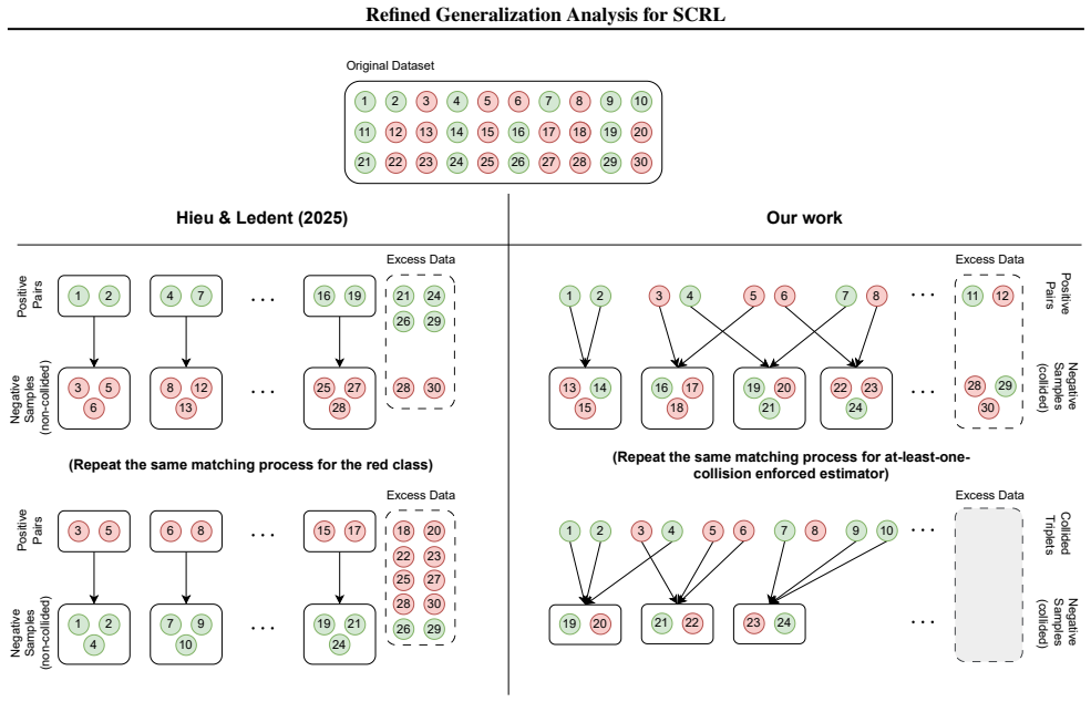
lnR/∆ N # , with probability of at least1−∆. 58 Refined Generalization Analysis for SCRL H. Refined Analysis for the EstimatorU hl N (f)from Hieu & Ledent (2025) To re-iterate from the main text, in Hieu & Ledent (2025), the estimator of the population contrastive risk is constructed for eachf∈ Fas follows: Uhl N (f) := RX r=1 bρrU r Θ(f)∀r∈[R] :U r Θ(f) ...

work page 2025
[47]

2bRT iidr (H) + 10B s ln 4/δ 2⌊Nr/2⌋ # (∗) ⩽ BR N + X r:Nr⩾2 bρr

¯X r u denotes theu th data-point in ¯Sr =S\S r. Remark H.2.For the sake of definition completeness, we define the empirical Rademacher complexity bRT iidr (H) = 0 whenT iid r =∅. In other words, the complexity is0when evaluated on an empty dataset. Theorem H.3(cf. Table 1).Let F be a class of representation functions and Uhl N (f) be defined for each f∈ ...

work page 2025
[48]

24CN(H) + 10B s 2 ln 12R ∆ #

We have the following result. Theorem H.6(Theorem H.5 without ρr ⩽ 1 2 assumption).Let F be a class of representation functions and let Uhl N (f) be defined for eachf∈ Fas in Eqn.(94). Then, for any∆∈(0,1), as long asN⩾ 2(k+1)2 1−ρmax ln 3R ∆ , we have: sup f∈F Uhl N (f)−L ϕ(f) ⩽ " 24CN(H) + 10B s 2 ln 12R ∆ #" bθ 1 2 k+2 r 2R N + (1− bθk+2) s k+ 1 N(1−ρ ...

work page arXiv 2025
[49]

sup g∈G 1 n nX i=1 g(zi)−Θ(g) # =E Sφ

or Bartlett et al. (2017, Lemma A.5)). Then, apply Massart’s finite lemma. The difference is that instead of using the standard Massart’s lemma for the regular notion of Rademacher Complexity (without absolute value), we apply Lemma L.4. Lemma L.6.(Hieu et al. (2024)) Let F be a class of representation functions f:X →R d and ℓ:R k →R + be a contrastive lo...

work page 2017