Recognition: no theorem link
Invariant domain preserving limiting of time explicit and time implicit discretizations for systems of conservation laws
Pith reviewed 2026-05-11 02:22 UTC · model grok-4.3
The pith
The limiting technique preserves invariant domains for high-order discretizations of conservation laws by expressing the solution as a convex combination of low-order invariant-domain-preserving states.
A machine-rendered reading of the paper's core claim, the machinery that carries it, and where it could break.
Core claim
By choosing limiting factors for the antidiffusive fluxes, the high-order discrete solution is expressed as a convex combination of invariant domain preserving quantities. This guarantees the limited solution lies inside all invariant domains whenever the low-order solution does. The construction applies to finite volume and discontinuous Galerkin spatial discretizations paired with explicit Runge-Kutta, implicit Runge-Kutta, or time discontinuous Galerkin integrators.
What carries the argument
Limiting coefficients for antidiffusive fluxes chosen to rewrite the high-order solution as a convex combination of invariant-domain-preserving quantities.
If this is right
- The scheme remains globally conservative because the flux limiting does not alter the telescoping sum.
- Formal accuracy order is preserved away from discontinuities or extrema.
- The same limiter works without change for explicit, implicit, and time-discontinuous time integrators.
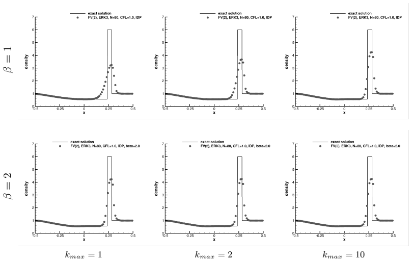
- Iterative limiting refines the result toward the high-order solution while enforcing domain preservation at each step.
Where Pith is reading between the lines
- The convex-combination structure may allow straightforward extension to additional invariant domains such as entropy inequalities.
- The acceleration heuristic could be analyzed for its effect on overall computational cost in stiff problems.
- Similar limiting ideas might apply to other discretizations that admit an antidiffusive flux decomposition.
Load-bearing premise
The existence of a computable low-order discretization that preserves all invariant domains, together with the ability to express the high-order solution through antidiffusive fluxes amenable to convex-combination limiting.
What would settle it
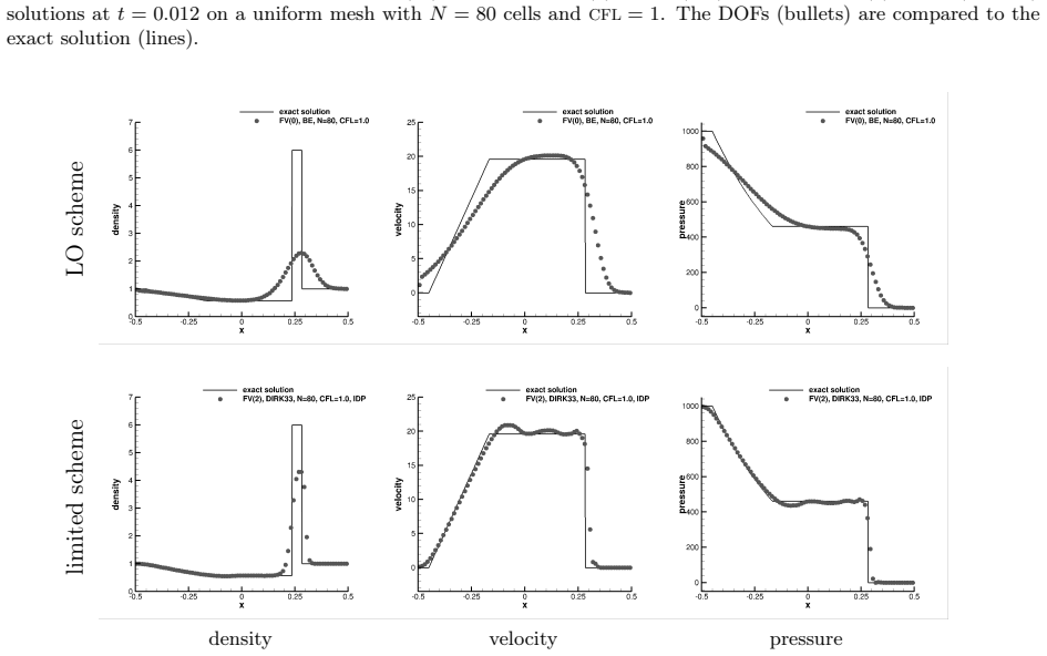
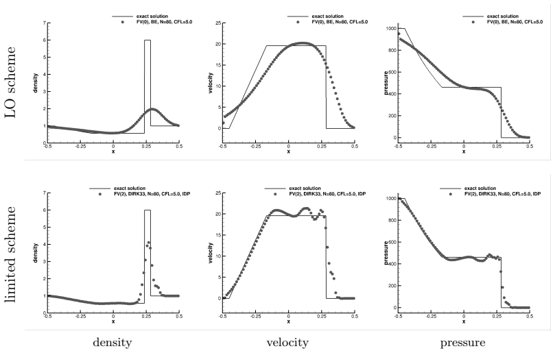
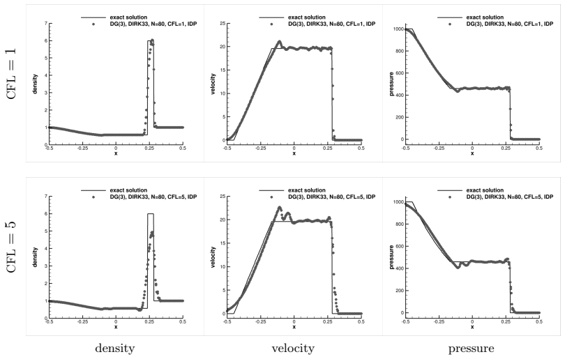
A specific test case such as a shock-tube problem for the Euler equations in which the limited solution produces a negative density or pressure even though the low-order solution does not.
Figures

read the original abstract
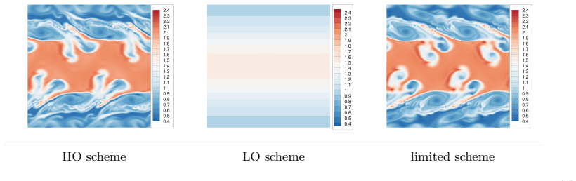
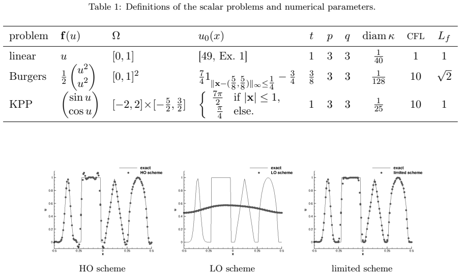
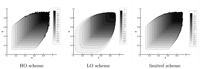
This work concerns the design and analysis of a limiting technique that allows the preservation of invariant domains for high-order numerical approximations of nonlinear hyperbolic systems of conservation laws. The method can be applied to any conservative discretization method in space as well as to a wide range of explicit and implicit time integration schemes. The method limits the high-order solution around a low-order accurate solution that is known to preserve all the invariant domains. It generalizes the flux-corrected transport limiter [J. P. Boris and D. L. Book, J. Comput. Phys., 11, 1973; S. T. Zalesak, J. Comput. Phys., 31, 1979] to systems of conservation laws and relies on the limitation of antidiffusive fluxes, but defines the limiting coefficients so as to express the limited solution as a convex combination of invariant domain preserving quantities similarly to the convex limiting framework [Guermond et al., Comput. Methods Appl. Mech. Engrg., 347, 2019]. We give details on the derivation of this limiting technique and provide some illustration with finite volume or discontinuous Galerkin (DG) space discretizations associated to explicit or implicit Runge-Kutta methods as well as to time DG integrations. The limiter is applied iteratively to refine the limited solution around the high-order one, while preserving the invariant domains, and a heuristic is proposed to accelerate its convergence. Numerical experiments solving one- and two-dimensional problems involving scalar hyperbolic equations and the compressible Euler equations are presented to illustrate the properties of these schemes.
Editorial analysis
A structured set of objections, weighed in public.
Referee Report
Summary. The manuscript develops a limiting technique to enforce invariant-domain preservation for high-order conservative discretizations of nonlinear hyperbolic systems. The method starts from any low-order IDP solution and limits antidiffusive fluxes so that the result is expressed as a convex combination of IDP states, generalizing both classical FCT and the convex-limiting framework. The construction is stated to apply to finite-volume and DG spatial discretizations paired with explicit or implicit Runge-Kutta integrators and with time-DG schemes. An iterative application of the limiter is proposed together with a convergence-acceleration heuristic, and the approach is illustrated on scalar advection and the compressible Euler equations in one and two space dimensions.
Significance. If the decomposition of an implicit high-order solution into a low-order IDP update plus exact antidiffusive increments can be performed without introducing consistency error or breaking telescoping conservation, the technique would constitute a useful extension of existing IDP limiting methods to implicit time discretizations, allowing high-order accuracy while retaining strict invariant-domain properties for systems such as the Euler equations.
major comments (2)
- [§3.3] §3.3 (implicit time discretization): the construction of the antidiffusive flux vector for a fully implicit Runge-Kutta or time-DG step is presented only after the nonlinear algebraic system has been solved. It is not shown that this post-hoc decomposition exactly recovers the original high-order update when the limiting coefficients are set to unity, nor that the limited fluxes remain conservative (i.e., that the telescoping property is preserved). Without this identity, the convex-combination argument does not guarantee that the limited solution satisfies the same conservation law as the unlimited one.
- [§4.1] §4.1 (iterative limiter): the iterative procedure is asserted to converge to an IDP state while staying close to the high-order solution, yet no a-priori bound on the number of iterations or proof that the fixed point remains conservative is supplied. The heuristic acceleration is described only numerically; its effect on the invariant-domain property must be verified analytically or by counter-example.
minor comments (2)
- [§2.2 and §3.3] Notation for the limiting coefficients α_{ij} is introduced in §2.2 but the dependence on the time-step index is not made explicit when the same symbols are reused for implicit schemes in §3.3; a uniform subscript convention would improve readability.
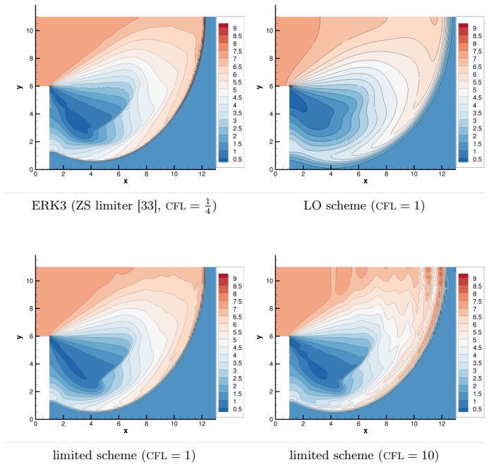
- [Figure 5] Figure 5 (two-dimensional Euler shock-tube): the caption does not state the polynomial degree of the DG approximation or the CFL number used for the implicit time step; these parameters are needed to reproduce the reported oscillation-free profiles.
Simulated Author's Rebuttal
We thank the referee for the careful reading and constructive comments. The two major points raised are addressed below with clarifications and planned revisions.
read point-by-point responses
-
Referee: [§3.3] §3.3 (implicit time discretization): the construction of the antidiffusive flux vector for a fully implicit Runge-Kutta or time-DG step is presented only after the nonlinear algebraic system has been solved. It is not shown that this post-hoc decomposition exactly recovers the original high-order update when the limiting coefficients are set to unity, nor that the limited fluxes remain conservative (i.e., that the telescoping property is preserved). Without this identity, the convex-combination argument does not guarantee that the limited solution satisfies the same conservation law as the unlimited one.
Authors: The antidiffusive flux vector is defined exactly as the difference between the already-computed high-order update and the low-order IDP update. Consequently, every limiting coefficient equal to one recovers the high-order solution by algebraic identity. Both the high-order and low-order updates are conservative (they satisfy the same telescoping property at the discrete level). Their difference therefore consists of increments whose global sum is zero, so the limited fluxes remain conservative. We will insert a short lemma in §3.3 that states this identity and the telescoping property explicitly. revision: yes
-
Referee: [§4.1] §4.1 (iterative limiter): the iterative procedure is asserted to converge to an IDP state while staying close to the high-order solution, yet no a-priori bound on the number of iterations or proof that the fixed point remains conservative is supplied. The heuristic acceleration is described only numerically; its effect on the invariant-domain property must be verified analytically or by counter-example.
Authors: Each iteration applies the same convex-limiting procedure around the fixed low-order IDP state, so every iterate is IDP by construction. Because the limiter is realized through conservative flux corrections, conservation is preserved at every step; the fixed point (when reached) therefore inherits both properties. We do not possess a general a-priori iteration bound, as the number depends on the mesh and the solution. The acceleration heuristic is purely numerical; we will add a short paragraph in §4.1 together with an additional numerical test that confirms the accelerated sequence remains IDP. revision: partial
Circularity Check
No significant circularity; derivation is self-contained via convex-combination properties
full rationale
The paper constructs a limiter by rewriting high-order updates (explicit or implicit) as a low-order IDP solution plus antidiffusive fluxes, then applies coefficients so the result is a convex combination of IDP states. This follows directly from the definition of convex combinations and the assumed existence of an IDP low-order scheme; no step reduces a claimed prediction or uniqueness result to a fitted parameter or self-citation by construction. Citations to Boris-Book, Zalesak, and Guermond et al. supply independent external support for the FCT and convex-limiting frameworks. The implicit decomposition is presented as an explicit algebraic construction within the method rather than an unverified assumption that collapses the invariance proof. The overall argument remains non-circular and externally falsifiable through the numerical experiments.
Axiom & Free-Parameter Ledger
axioms (2)
- domain assumption Low-order discretizations exist that preserve all invariant domains for the systems considered
- standard math Convex combinations of states inside an invariant domain remain inside the domain
Reference graph
Works this paper leans on
- [1]
-
[2]
Serre, Domaines invariants pour les systèmes hyperboliques de lois de conservation, J
D. Serre, Domaines invariants pour les systèmes hyperboliques de lois de conservation, J. Differ. Equ. 69 (5) (1987) 46–62.doi:10.1016/0022-0396(87)90102-1
-
[3]
Hoff, Invariant regions for systems of conservation laws, Trans
D. Hoff, Invariant regions for systems of conservation laws, Trans. Amer. Math. Soc. 289 (1985) 591–610.doi:https://doi.org/10.2307/2000254
-
[4]
Kružkov, First order quasilinear equations in several independent variables, Math
S. Kružkov, First order quasilinear equations in several independent variables, Math. Ussr Sbornik 10 (1970) 217–243
work page 1970
-
[5]
H. Frid, Maps of convex sets and invariant regions for finite-difference systems of conserva- tion laws, Arch. Rational Mech. Anal. 160 (2001) 245–269.doi:https://doi.org/10.1007/ s002050100166
work page 2001
-
[6]
J.-L. Guermond, B. Popov, Invariant domains and first-order continuous finite element ap- proximation for hyperbolic systems, SIAM J. Numer. Anal. 54 (4) (2016) 2466–2489.doi: 10.1137/16M1074291
-
[7]
R.Löhner, K.Morgan, J.Peraire, M.Vahdati, Finiteelementflux-correctedtransport(fem–fct) for the euler and navier–stokes equations, Int. J. Numer. Meth. Fluids 7 (10) (1987) 1093–1109. doi:https://doi.org/10.1002/fld.1650071007
-
[8]
J. P. Boris, D. L. Book, Flux-corrected transport. I. SHASTA, a fluid transport algorithm that works, J. Comput. Phys. 11 (1) (1973) 38–69.doi:10.1016/0021-9991(73)90147-2
-
[9]
S. T. Zalesak, Fully multidimensional flux-corrected transport algorithms for fluids, J. Comput. Phys. 31 (3) (1979) 335–362.doi:https://doi.org/10.1016/0021-9991(79)90051-2
-
[10]
D. Kuzmin, S. Turek, Flux correction tools for finite elements, J. Comput. Phys. 175 (2) (2002) 525–558.doi:https://doi.org/10.1006/jcph.2001.6955. 30
-
[11]
F. Renac, Maximum principle preserving and entropy stable time implicit DGSEM for non- linear scalar conservation laws, ESAIM: Math. Model. Numer. Anal. 59 (5) (2025) 2583–2612. doi:10.1051/m2an/2025070
-
[12]
R. Milani, F. Renac, J. Ruel, Maximum principle preserving time implicit DGSEM for linear scalar hyperbolic conservation laws, J. Comput. Phys. 514 (2024) 113254.doi:10.1016/j. jcp.2024.113254
work page doi:10.1016/j 2024
-
[13]
J.-L. Guermond, B. Popov, I. Tomas, Invariant domain preserving discretization-independent schemes and convex limiting for hyperbolic systems, Comput. Methods Appl. Mech. Engrg. 347 (2019) 143–175.doi:https://doi.org/10.1016/j.cma.2018.11.036
-
[14]
J.-L. Guermond, M. Nazarov, B. Popov, I. Tomas, Second-order invariant domain preserving approximation of the Euler equations using convex limiting, SIAM J. Sci. Comput. 40 (5) (2018) A3211–A3239.doi:10.1137/17M1149961
-
[15]
W. Pazner, Sparse invariant domain preserving discontinuous Galerkin methods with subcell convex limiting, Comput. Methods Appl. Mech. Engrg. 382 (2021) 113876.doi:https://doi. org/10.1016/j.cma.2021.113876
-
[16]
D. Kuzmin, Monolithic convex limiting for continuous finite element discretizations of hyper- bolic conservation laws, Comput. Methods. Appl. Mech. Eng. 361 (2020) 112804.doi:https: //doi.org/10.1016/j.cma.2019.112804
-
[17]
P. Moujaes, D. Kuzmin, Monolithic convex limiting and implicit pseudo-time stepping for calculating steady-state solutions of the Euler equations, J. Comput. Phys. 523 (2025) 113687. doi:https://doi.org/10.1016/j.jcp.2024.113687
-
[18]
J. Qiu, B. C. Khoo, C.-W. Shu, A numerical study for the performance of the Runge-Kutta discontinuous Galerkin method based on different numerical fluxes, J. Comput. Phys. 212 (2) (2006) 540–565.doi:https://doi.org/10.1016/j.jcp.2005.07.011
-
[19]
F. Renac, Stationary discrete shock profiles for scalar conservation laws with a discontinuous Galerkin method, SIAM J. Numer. Anal. 53 (4) (2015) 1690–1715.doi:10.1137/14097906X
-
[20]
R. Moura, G. Mengaldo, J. Peiró, S. Sherwin, On the eddy-resolving capability of high-order discontinuous Galerkin approaches to implicit LES / under-resolved DNS of Euler turbulence, J. Comput. Phys. 330 (2017) 615–623.doi:https://doi.org/10.1016/j.jcp.2016.10.056
-
[21]
J.-B. Chapelier, M. de la Llave Plata, F. Renac, E. Lamballais, Evaluation of a high-order discontinuous Galerkin method for the DNS of turbulent flows, Comput. Fluids 95 (2014) 210–226.doi:10.1016/j.compfluid.2014.02.015
-
[22]
C. Schär, P. K. Smolarkiewicz, A synchronous and iterative flux-correction formalism for cou- pled transport equations, J. Comput. Phys. 128 (1) (1996) 101–120.doi:https://doi.org/ 10.1006/jcph.1996.0198
-
[23]
Kuzmin, Explicit and implicit FEM-FCT algorithms with flux linearization, J
D. Kuzmin, Explicit and implicit FEM-FCT algorithms with flux linearization, J. Comput. Phys. 228 (7) (2009) 2517–2534.doi:https://doi.org/10.1016/j.jcp.2008.12.011. 31
-
[24]
E. Godlewski, P.-A. Raviart, Hyperbolic systems of conservation laws, no. 3-4, Ellipses, 1991
work page 1991
-
[25]
J. van der Vegt, H. van der Ven, Space–time discontinuous Galerkin finite element method with dynamic grid motion for inviscid compressible flows: I. general formulation, J. Comput. Phys. 182 (2) (2002) 546–585.doi:https://doi.org/10.1006/jcph.2002.7185
-
[26]
T. J. Barth, Simplified discontinuous Galerkin methods for systems of conservation laws with convex extension, in: B. Cockburn, G. E. Karniadakis, C.-W. Shu (Eds.), Discontinuous Galerkin Methods, Springer Berlin Heidelberg, Berlin, Heidelberg, 2000, pp. 63–75
work page 2000
- [27]
-
[28]
C. Ollivier-Gooch, M. Van Altena, A high-order-accurate unstructured mesh finite-volume scheme for the advection–diffusion equation, J. Comput. Phys. 181 (2) (2002) 729–752.doi: https://doi.org/10.1006/jcph.2002.7159
-
[29]
F. Haider, J.-P. Croisille, B. Courbet, Stability analysis of the cell centered finite-volume MUSCL method on unstructured grids, Numer. Math. 113 (2009) 555–600.doi:https:// doi.org/10.1007/s00211-009-0242-6
-
[30]
G. Pont, P. Brenner, P. Cinnella, B. Maugars, J.-C. Robinet, Multiple-correction hybrid k- exact schemes for high-order compressible RANS-LES simulations on fully unstructured grids, J. Comput. Phys. 350 (2017) 45–83.doi:https://doi.org/10.1016/j.jcp.2017.08.036
-
[31]
H.-Z. Tang, K. Xu, Positivity-preserving analysis of explicit and implicit Lax-Friedrichs schemes for compressible Euler equations, J. Sci. Comput. 15 (1) (2000) 19–28.doi:https: //doi.org/10.1023/A:1007593601466
-
[32]
R. Eymard, T. Gallouët, R. Herbin, Finite volume methods, in: Solution of Equation inRn (Part 3), Techniques of Scientific Computing (Part 3), Vol. 7 of Handbook of Numerical Anal- ysis, Elsevier, 2000, pp. 713–1018.doi:https://doi.org/10.1016/S1570-8659(00)07005-8
-
[33]
X. Zhang, C.-W. Shu, On positivity-preserving high order discontinuous Galerkin schemes for compressible Euler equations on rectangular meshes, J. Comput. Phys. 229 (23) (2010) 8918–8934
work page 2010
-
[34]
X. Zhang, C.-W. Shu, On maximum-principle-satisfying high order schemes for scalar conser- vation laws, J. Comput. Phys. 229 (9) (2010) 3091–3120
work page 2010
-
[35]
T. C. Fisher, M. H. Carpenter, High-order entropy stable finite difference schemes for nonlinear conservation laws: Finite domains, J. Comput. Phys. 252 (2013) 518–557
work page 2013
-
[36]
G. J. Gassner, A skew-symmetric discontinuous Galerkin spectral element discretization and its relation to SBP-SAT finite difference methods, SIAM J. Sci. Comput. 35 (3) (2013) A1233– A1253.doi:10.1137/120890144
-
[37]
D. A. Kopriva, Metric identities and the discontinuous spectral element method on curvi- linear meshes., J. Sci. Comput. 26 (2006) 302–327.doi:https://doi.org/10.1007/ s10915-005-9070-8. 32
work page 2006
-
[38]
Jameson, Positive schemes and shock modelling for compressible flows, Int
A. Jameson, Positive schemes and shock modelling for compressible flows, Int. J. Numer. Meth. Fluids 20 (8-9) (1995) 743–776.doi:https://doi.org/10.1002/fld.1650200805
-
[39]
F. Renac, M. de la Llave Plata, E. Martin, J. B. Chapelier, V. Couaillier, Aghora: A High- Order DG Solver for Turbulent Flow Simulations, Springer International Publishing, 2015, pp. 315–335.doi:10.1007/978-3-319-12886-3_15
-
[40]
Rusanov, Calculation of interaction of non-steady shock waves with obstacles, J
V. Rusanov, Calculation of interaction of non-steady shock waves with obstacles, J. Comp. Math. Phys. USSR 1 (1961) 267–279
work page 1961
-
[41]
R. Löhner, Applied computational fluid dynamics techniques: an introduction based on finite element methods, John Wiley & Sons, 2008
work page 2008
-
[42]
C.-W. Shu, S. Osher, Efficient implementation of essentially non-oscillatory shock-capturing schemes, J. Comput. Phys. 77 (2) (1988) 439–471
work page 1988
-
[43]
Alexander, Diagonally implicit Runge–Kutta methods for stiff O.D.E.’s, SIAM J
R. Alexander, Diagonally implicit Runge–Kutta methods for stiff O.D.E.’s, SIAM J. Numer. Anal. 14 (6) (1977) 1006–1021.doi:10.1137/0714068
-
[44]
E. F. Toro, Riemann Solvers and Numerical Methods for Fluid Dynamics: A Practical Intro- duction. Third Edition, Springer-Verlag Berlin Heidelberg, 2009
work page 2009
-
[45]
P. Chandrashekar, Kinetic energy preserving and entropy stable finite volume schemes for com- pressibleEulerandNavier-Stokesequations, Commun.Comput.Phys.14(5)(2013)1252–1286. doi:10.4208/cicp.170712.010313a
-
[46]
J. Chan, H. Ranocha, A. M. Rueda-Ramírez, G. J. Gassner, T. Warburton, On the entropy projection and the robustness of high order entropy stable discontinuous Galerkin schemes for under-resolved flows, Frontiers in Physics 10 (2022).doi:10.3389/fphy.2022.898028
-
[47]
V. Carlier, F. Renac, Invariant domain preserving high-order spectral discontinuous ap- proximations of hyperbolic systems, SIAM J. Sci. Comput. 45 (3) (2023) A1385–A1412. doi:10.1137/22M1492015
-
[48]
P. Woodward, P. Colella, The numerical simulation of two-dimensional fluid flow with strong shocks, J. Comput. Phys. 54 (1) (1984) 115–173.doi:https://doi.org/10.1016/ 0021-9991(84)90142-6
work page 1984
-
[49]
Efficient Implementation of Weighted ENO Schemes
G.-S. Jiang, C.-W. Shu, Efficient implementation of weighted ENO schemes, J. Comput. Phys. 126 (1) (1996) 202–228.doi:https://doi.org/10.1006/jcph.1996.0130
-
[50]
R. J. LeVeque, Finite Volume Methods for Hyperbolic Problems, Cambridge Texts in Applied Mathematics, Cambridge University Press, 2002
work page 2002
-
[51]
J.-L. Guermond, B. Popov, Invariant domains and second-order continuous finite element approximation for scalar conservation equations, SIAM J. Numer. Anal. 55 (6) (2017) 3120– 3146.doi:10.1137/16M1106560
-
[52]
A. Kurganov, G. Petrova, B. Popov, Adaptive semidiscrete central-upwind schemes for nonconvex hyperbolic conservation laws, SIAM J. Sci. Comput. 29 (6) (2007) 2381–2401. doi:10.1137/040614189. 33
discussion (0)
Sign in with ORCID, Apple, or X to comment. Anyone can read and Pith papers without signing in.