arxiv: 2605.08344 · v1 · submitted 2026-05-08 · 💻 cs.LG

Recognition: 2 theorem links

· Lean Theorem

What Time Is It? How Data Geometry Makes Time Conditioning Optional for Flow Matching

Alec Helbling , Sebastian Gutierrez Hernandez , Benjamin Hoover , Duen Horng Chau , Parikshit Ram

Authors on Pith no claims yet

Pith reviewed 2026-05-12 00:54 UTC · model grok-4.3

classification 💻 cs.LG

keywords flow matchingtime conditioningdata geometrycoupling variancetime-blind trainingspiked covariancegenerative modelsinterpolation time

0 comments

The pith

High-dimensional data geometry allows recovering interpolation time from a single noisy observation, rendering explicit time conditioning optional in flow matching.

A machine-rendered reading of the paper's core claim, the machinery that carries it, and where it could break.

The paper decomposes the time-blind flow matching loss into two irreducible errors: coupling variance from ambiguous noise-data pairings and the time-blindness gap from ignoring time. It shows that the gap is strictly positive yet becomes asymptotically negligible when data concentrates near a low-dimensional subspace. Using a spiked-covariance model, the authors derive a closed-form estimator that recovers time at rate O(1/sqrt(d-k)) from orthogonal noise directions. This resolves why time-blind models succeed in practice on high-dimensional data. Experiments on image datasets further show that changing the coupling affects loss and quality far more than removing time conditioning.

Core claim

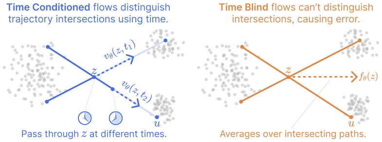
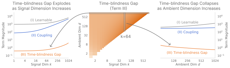
Decomposing the time-blind flow matching loss identifies coupling variance and the time-blindness gap. When data concentrates near a k-dimensional subspace, time can be recovered from the statistical structure of noisy interpolants in directions orthogonal to the data; under a spiked-covariance model, this yields a closed-form estimator that recovers t from a single observation z at rate O(1/sqrt(d-k)) for ambient dimension d. As a consequence, the time-blindness gap is asymptotically negligible relative to the coupling variance.

What carries the argument

The closed-form estimator for interpolation time t derived from the spiked-covariance model using directions orthogonal to the data subspace.

If this is right

Time-blind training incurs only asymptotically negligible extra error compared to time-conditioned training in high dimensions.
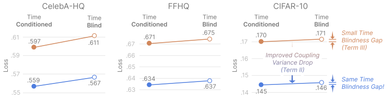
The choice of coupling between noise and data points has a larger impact on model performance than including or removing time conditioning.
Time is statistically identifiable from data geometry without explicit conditioning.
Empirical results on CIFAR-10, CelebA-HQ, and FFHQ confirm that coupling changes affect loss and sample quality more than time removal.

Where Pith is reading between the lines

These are editorial extensions of the paper, not claims the author makes directly.

Similar geometry-based identifiability may extend to other interpolation-based generative models.
Practitioners could prioritize optimizing couplings over adding time-conditioning networks.
The result suggests testing the estimator on structured or lower-dimensional data to find where identifiability breaks.
Extensions to non-Gaussian noise could broaden the applicability of time recovery.

Load-bearing premise

Real data concentrates near a k-dimensional subspace, allowing time to be recovered from orthogonal noise directions under the spiked-covariance model.

What would settle it

Computing the time estimator on high-dimensional datasets like images and checking whether recovery error decreases at rate O(1/sqrt(d-k)), or observing that time removal degrades performance more than coupling changes when the subspace concentration fails.

Figures

Figures reproduced from arXiv: 2605.08344 by Alec Helbling, Benjamin Hoover, Duen Horng Chau, Parikshit Ram, Sebastian Gutierrez Hernandez.

**Figure 1.** Figure 1: Time-blind flow matching works because data and noise occupy subspaces of very different sizes, leaving a large residual noise subspace whose variance encodes the interpolation time. (Left) Noise dominates in a large subspace: the source ε ∼ N (0, Id) is isotropic over the full ambient dimension d. (Right) Data concentrates in a small subspace: the target distribution is supported on a k-dimensional signal… view at source ↗

**Figure 2.** Figure 2: Time-conditioned flows disambiguate trajectory intersections using t. Time-blind flows must commit to a single velocity at each location, averaging over conflicting trajectories. (Left) A time-conditioned model vθ(z, t) observes t and can assign different velocities at the same spatial location z for different times; here, vθ(z, 0.3) and vθ(z, 0.7) point along distinct trajectories that pass through z. (Ri… view at source ↗

**Figure 3.** Figure 3: Real data concentrates in a low-rank subspace and leaves a sizable residual subspace. Cumulative explained variance captured by the top-k principal components on each real dataset and on the spiked covariance model used in Theorem 2. Pixel-space CIFAR-10 shows dramatic low-rank concentration; on the FFHQ and CelebA-HQ VAE latents variance is more spread out across components but still concentrates most of … view at source ↗

**Figure 4.** Figure 4: The error decomposition is additive and coupling-dominated. Shown are converged test-set MSE for each ablation. OT coupling, time-conditioned (•); OT coupling, time-blind (◦); naive coupling, time-conditioned (•); naive coupling, time-blind (◦). The large vertical drop between lines is the coupling variance (Term II); the small horizontal gap within each line is the time-blindness gap (Term III). On both d… view at source ↗

**Figure 5.** Figure 5: Empirical estimates of t on real datasets are precise and match the theoretically predicted bound. Distribution of estimation error tˆ− t for the noise-subspace estimator across four settings: a synthetic spiked covariance model, CIFAR-10 (pixel space), FFHQ (VAE latent), and CelebA-HQ (VAE latent), with k chosen at the 95% explained-variance threshold per dataset. Empirical (solid) closely matches the the… view at source ↗

**Figure 6.** Figure 6: The time-blindness gap is governed by d − k and dwarfed by the coupling variance. (Left) Growing k at fixed d = 1024 inflates both the gap and the coupling loss. (Center) Heatmap of the gap magnitude across the (d, k) plane. (Right) Growing d at fixed k = 64 collapses the gap. this behavior from data, including convolutional, self-supervised, and real-image blind-denoising methods [10, 2, 32]. These works … view at source ↗

read the original abstract

Recent work has shown that models flow matching models can be trained without explicit time conditioning, challenging the standard view that the interpolation time is needed to disambiguate velocity targets. But why should a time-blind model work at all? Decomposing the time-blind flow matching loss, we identify two sources of irreducible error: a coupling variance, which arises from ambiguous velocity targets induced by how noise and data points are paired, and the time-blindness gap, which is the additional error caused by ignoring time. This gap shows that time-blind training is strictly harder than conventional training, reinforcing the puzzle that time-blind models work so well in practice. We resolve this tension by showing that the geometry of high-dimensional data makes time identifiable directly from noisy observations. When data concentrates near a $k$-dimensional subspace, time can be recovered from the statistical structure of noisy interpolants in directions orthogonal to the data; under a spiked-covariance model, this yields a closed-form estimator that recovers $t$ from a single observation $z$ at rate $O(1/\sqrt{d-k})$ for ambient dimension $d$. As a consequence, we prove that the time-blindness gap is asymptotically negligible relative to the coupling variance. We empirically demonstrate our identifiability result on real-world data and show that changing the coupling has a much larger effect on loss and sample quality than removing time conditioning across CIFAR-10, CelebA-HQ, and FFHQ. These results explain why time-blind flow matching works and show that the main practical lever is the choice of coupling, not explicit time conditioning.

Editorial analysis

A structured set of objections, weighed in public.

Desk editor's note, referee report, simulated authors' rebuttal, and a circularity audit. Tearing a paper down is the easy half of reading it; the pith above is the substance, this is the friction.

Desk Editor's Note private letter to a colleague

The paper shows time-blind flow matching works because data subspace geometry lets you recover t from orthogonal noise at rate O(1/sqrt(d-k)) under spiked covariance, making the time-blindness gap asymptotically smaller than coupling variance, with experiments confirming coupling choice matters more.

read the letter

The main takeaway is that explicit time conditioning is often unnecessary in flow matching because high-dimensional data geometry makes the interpolation time recoverable from a single noisy sample. The paper also finds that the choice of coupling between noise and data points has a larger effect on training loss and sample quality than whether time is conditioned on or not. They reach this by decomposing the time-blind loss into coupling variance from ambiguous pairings and an extra time-blindness gap from dropping the time input. Under the assumption that data concentrates near a k-dimensional subspace, they show t can be identified from the statistical structure in the orthogonal directions. With a spiked-covariance model they derive a closed-form estimator that recovers t at rate O(1/sqrt(d-k)) for ambient dimension d, and they prove the time-blindness gap becomes negligible relative to coupling variance as d grows. On the empirical side they check identifiability on CIFAR-10, CelebA-HQ, and FFHQ and run ablations that swap couplings while toggling time conditioning, showing the coupling change dominates. The decomposition is straightforward and useful for explaining why these models succeed without time inputs. The identifiability argument and the asymptotic comparison are new relative to the cited prior work, and the experiments give a clear practical message that coupling is the lever to tune. The main soft spot is the spiked-covariance assumption required for the closed-form estimator and the negligibility proof. Real image covariances usually show gradual power-law eigenvalue decay rather than a sharp drop after k large ones, so the stated recovery rate and the claim that the gap vanishes may not hold at the same strength. The paper does provide empirical checks on real data, but those do not directly test whether the theoretical rate explains the observations. The free parameter k also requires selection in practice. This work is aimed at researchers working on flow matching and related generative models who want to simplify conditioning or understand why certain shortcuts succeed. A reader focused on the theory of these models or on reducing training overhead would find the loss breakdown and geometry argument worth their time. It deserves a serious referee because the question is practically relevant, the decomposition is clean, and the experiments are on standard benchmarks, even though the covariance assumption will need scrutiny. I would send it to peer review.

Referee Report

2 major / 2 minor

Summary. The paper decomposes the time-blind flow matching loss into a coupling variance term (from ambiguous velocity targets due to noise-data pairings) and a time-blindness gap (additional error from ignoring time). It proves that under a spiked-covariance model where data concentrates near a k-dimensional subspace, time t is identifiable from a single noisy interpolant z via a closed-form estimator exploiting orthogonal noise directions, at rate O(1/sqrt(d-k)). This makes the time-blindness gap asymptotically negligible relative to coupling variance. Empirically, the authors show identifiability on image datasets and that varying the coupling affects loss and sample quality more than removing time conditioning on CIFAR-10, CelebA-HQ, and FFHQ.

Significance. If the asymptotic negligibility holds under the model's assumptions, the work provides a geometric explanation for the practical success of time-blind flow matching, shifting emphasis to coupling choice as the primary lever. The closed-form estimator and proof of negligibility relative to coupling variance are notable strengths, as is the empirical demonstration across standard generative modeling benchmarks. This could simplify training pipelines for flow-based models while clarifying when explicit time conditioning is redundant.

major comments (2)

[§3] §3 (spiked-covariance model and closed-form estimator): The proof that the time-blindness gap vanishes asymptotically relative to coupling variance relies on the assumption of k large eigenvalues with the remainder exactly equal (spiked model). Real image covariances typically exhibit gradual power-law spectral decay rather than a sharp cutoff; this mismatch risks that the O(1/sqrt(d-k)) recovery rate does not hold, so the negligibility claim may not transfer to the datasets used in the experiments.
[§4] Theorem on asymptotic negligibility (likely §4): while the derivation is internally consistent under the spiked model, the paper does not provide a robustness analysis or bound on estimator bias/variance when eigenvalues decay continuously. This is load-bearing for the central claim that geometry makes time conditioning optional in practice.

minor comments (2)

The role of the free parameter k (subspace dimension) in the estimator should be clarified in the main text, including how it is chosen or estimated for the real-data experiments.
Figure captions for the empirical identifiability plots could more explicitly state the metric used to measure time recovery accuracy.

Simulated Author's Rebuttal

2 responses · 0 unresolved

We thank the referee for their constructive feedback and positive evaluation of the paper's contributions. We respond to the major comments point by point below, indicating planned revisions where appropriate.

read point-by-point responses

Referee: [§3] §3 (spiked-covariance model and closed-form estimator): The proof that the time-blindness gap vanishes asymptotically relative to coupling variance relies on the assumption of k large eigenvalues with the remainder exactly equal (spiked model). Real image covariances typically exhibit gradual power-law spectral decay rather than a sharp cutoff; this mismatch risks that the O(1/sqrt(d-k)) recovery rate does not hold, so the negligibility claim may not transfer to the datasets used in the experiments.

Authors: We agree that the spiked model is a simplifying assumption that enables the closed-form estimator and the explicit convergence rate. Real-world data covariances do exhibit power-law decay rather than a sharp cutoff after k dimensions. However, the identifiability result fundamentally depends on the data having a low effective dimensionality, which is captured by the spiked model as an approximation. In the experiments, we select k based on the point where the eigenvalue spectrum flattens, which is observable even in gradual decay cases. We will revise §3 to include a brief analysis of the eigenvalue spectra for the image datasets and discuss how the estimator remains effective. This should clarify the applicability to the empirical settings. revision: partial
Referee: [§4] Theorem on asymptotic negligibility (likely §4): while the derivation is internally consistent under the spiked model, the paper does not provide a robustness analysis or bound on estimator bias/variance when eigenvalues decay continuously. This is load-bearing for the central claim that geometry makes time conditioning optional in practice.

Authors: The referee correctly notes that the asymptotic negligibility is proven under the spiked model. A full robustness analysis for continuously decaying eigenvalues would indeed bolster the central claim. We will add to the revised manuscript a discussion on the sensitivity of the estimator to deviations from the spiked assumption, including a bound on the additional variance introduced by bulk eigenvalue decay. This will be supported by numerical simulations on synthetic data with power-law spectra. We believe this addresses the concern while preserving the main theoretical result. revision: yes

Circularity Check

0 steps flagged

No circularity: derivation is conditional on explicit spiked-covariance assumption

full rationale

The paper's central result derives a closed-form t estimator and proves asymptotic negligibility of the time-blindness gap directly from the stated spiked-covariance model (k large eigenvalues, remainder equal) and high-dimensional geometry. The estimator is obtained by algebraic manipulation of the orthogonal noise directions under this model, not by fitting to the flow-matching loss or target metric. No self-citations are invoked as load-bearing premises, no ansatz is smuggled, and no prediction is renamed from a fitted input. The proof is therefore self-contained as a conditional mathematical statement; the strength of the spiked model is a modeling assumption open to empirical scrutiny but does not create circularity within the derivation chain.

Axiom & Free-Parameter Ledger

1 free parameters · 2 axioms · 0 invented entities

The central claim rests on the domain assumption that data concentrates near a low-dimensional subspace and on the spiked-covariance model chosen to obtain a closed-form estimator; both are standard in high-dimensional statistics but are load-bearing here.

free parameters (1)

k (subspace dimension)
Dimension of the subspace near which data is assumed to concentrate; determines the rate O(1/sqrt(d-k)).

axioms (2)

domain assumption Data concentrates near a k-dimensional subspace
Invoked to show that time can be recovered from noise statistics in the orthogonal complement.
domain assumption Spiked-covariance model governs the data distribution
Used to derive the closed-form estimator that recovers t at rate O(1/sqrt(d-k)).

pith-pipeline@v0.9.0 · 5601 in / 1385 out tokens · 47774 ms · 2026-05-12T00:54:58.084277+00:00 · methodology

discussion (0)

Lean theorems connected to this paper

Citations machine-checked in the Pith Canon. Every link opens the source theorem in the public Lean library.

IndisputableMonolith/Cost/FunctionalEquation.lean washburn_uniqueness_aczel unclear

?

unclear
Relation between the paper passage and the cited Recognition theorem.

Under the spiked covariance model, the residual-subspace energy of a single interpolant z yields a closed-form estimator of t with error O_p(1/sqrt(d-k)) (Theorem 2).
IndisputableMonolith/Foundation/RealityFromDistinction.lean reality_from_one_distinction unclear

?

unclear
Relation between the paper passage and the cited Recognition theorem.

the time-blindness gap is asymptotically negligible relative to the coupling variance

What do these tags mean?

matches: The paper's claim is directly supported by a theorem in the formal canon.
supports: The theorem supports part of the paper's argument, but the paper may add assumptions or extra steps.
extends: The paper goes beyond the formal theorem; the theorem is a base layer rather than the whole result.
uses: The paper appears to rely on the theorem as machinery.
contradicts: The paper's claim conflicts with a theorem or certificate in the canon.
unclear: Pith found a possible connection, but the passage is too broad, indirect, or ambiguous to say the theorem truly supports the claim.

Reference graph

Works this paper leans on

35 extracted references · 35 canonical work pages · 5 internal anchors

[1]

Building Normalizing Flows with Stochastic Interpolants

Michael S. Albergo and Eric Vanden-Eijnden. Building normalizing flows with stochastic interpolants, 2023. URLhttps://arxiv.org/abs/2209.15571

work page internal anchor Pith review arXiv 2023
[2]

Noise2Self: Blind denoising by self-supervision

Joshua Batson and Loic Royer. Noise2Self: Blind denoising by self-supervision. In Kamalika Chaudhuri and Ruslan Salakhutdinov, editors,Proceedings of the 36th International Conference on Machine Learning, volume 97 ofProceedings of Machine Learning Research, pages 524–533. PMLR, 2019. URLhttps://proceedings.mlr.press/v97/batson19a.html

work page 2019
[3]

Polar factorization and monotone rearrangement of vector-valued functions , url =

Yann Brenier. Polar factorization and monotone rearrangement of vector-valued functions. Communications on Pure and Applied Mathematics, 44(4):375–417, 1991. doi: https://doi. org/10.1002/cpa.3160440402. URL https://onlinelibrary.wiley.com/doi/abs/10. 1002/cpa.3160440402

work page doi:10.1002/cpa.3160440402 1991
[4]

Bradley C. A. Brown, Anthony L. Caterini, Brendan Leigh Ross, Jesse C. Cresswell, and Gabriel Loaiza-Ganem. Verifying the union of manifolds hypothesis for image data. InInternational Conference on Learning Representations, 2023. URL https://openreview.net/forum? id=Rvee9CAX4fi

work page 2023
[5]

An efficient statistical method for image noise level estimation

Guangyong Chen, Fengyuan Zhu, and Pheng Ann Heng. An efficient statistical method for image noise level estimation. InProceedings of the IEEE International Conference on Computer Vision (ICCV), pages 477–485, 2015

work page 2015
[6]

Score approximation, estimation and distribution recovery of diffusion models on low-dimensional data

Minshuo Chen, Kaixuan Huang, Tuo Zhao, and Mengdi Wang. Score approximation, estimation and distribution recovery of diffusion models on low-dimensional data. InProceedings of the 40th International Conference on Machine Learning, 2023. URL https://arxiv.org/abs/ 2302.07194

work page arXiv 2023
[7]

Diffusion models beat GANs on image synthesis

Prafulla Dhariwal and Alexander Nichol. Diffusion models beat GANs on image synthesis. In Advances in Neural Information Processing Systems, volume 34, pages 8780–8794, 2021

work page 2021
[8]

Journal of the American Statistical Association106(496), 1602– 1614 (2011)

Bradley Efron. Tweedie’s formula and selection bias.Journal of the American Statistical Association, 106(496):1602–1614, 2011. doi: 10.1198/jasa.2011.tm11181

work page doi:10.1198/jasa.2011.tm11181 2011
[9]

Unbalanced minibatch optimal transport; applications to domain adaptation

Kilian Fatras, Thibault Sejourne, Nicolas Courty, and Rémi Flamary. Unbalanced minibatch optimal transport; applications to domain adaptation. In Marina Meila and Tong Zhang, editors,Proceedings of the 38th International Conference on Machine Learning, volume 139 of Proceedings of Machine Learning Research, pages 3186–3197. PMLR, 18–24 Jul 2021. URL https...

work page 2021
[10]

Toward convolutional blind denoising of real photographs

Shi Guo, Zifei Yan, Kai Zhang, Wangmeng Zuo, and Lei Zhang. Toward convolutional blind denoising of real photographs. InProceedings of the IEEE/CVF Conference on Computer Vision and Pattern Recognition, pages 1712–1722, 2019

work page 2019
[11]

Hénaff, Johannes Ballé, Neil C

Olivier J. Hénaff, Johannes Ballé, Neil C. Rabinowitz, and Eero P. Simoncelli. The local low- dimensionality of natural images. InInternational Conference on Learning Representations,

work page
[12]

URLhttps://arxiv.org/abs/1412.6626

work page arXiv
[13]

Johnstone

Iain M. Johnstone. On the distribution of the largest eigenvalue in principal components analysis. The Annals of Statistics, 29(2):295–327, 2001. doi: 10.1214/aos/1009210544

work page doi:10.1214/aos/1009210544 2001
[14]

Blind denoising diffusion models and the blessings of dimensionality, 2026

Zahra Kadkhodaie, Aram-Alexandre Pooladian, Sinho Chewi, and Eero Simoncelli. Blind denoising diffusion models and the blessings of dimensionality, 2026. URL https://arxiv. org/abs/2602.09639. 10

work page arXiv 2026
[15]

Progressive growing of gans for improved quality, stability, and variation, 2018

Tero Karras, Timo Aila, Samuli Laine, and Jaakko Lehtinen. Progressive growing of gans for improved quality, stability, and variation, 2018. URL https://arxiv.org/abs/1710. 10196

work page 2018
[16]

A style-based generator architecture for generative adversarial networks

Tero Karras, Samuli Laine, and Timo Aila. A style-based generator architecture for generative adversarial networks, 2019. URLhttps://arxiv.org/abs/1812.04948

work page arXiv 2019
[17]

Learning multiple layers of features from tiny images

Alex Krizhevsky. Learning multiple layers of features from tiny images. Technical report, University of Toronto, 2009

work page 2009
[18]

Yaron Lipman, Ricky T. Q. Chen, Heli Ben-Hamu, Maximilian Nickel, and Matt Le. Flow matching for generative modeling, 2023. URLhttps://arxiv.org/abs/2210.02747

work page internal anchor Pith review Pith/arXiv arXiv 2023
[19]

Flow Straight and Fast: Learning to Generate and Transfer Data with Rectified Flow

Xingchao Liu, Chengyue Gong, and Qiang Liu. Flow straight and fast: Learning to generate and transfer data with rectified flow, 2022. URLhttps://arxiv.org/abs/2209.03003

work page internal anchor Pith review Pith/arXiv arXiv 2022
[20]

Single-image noise level estimation for blind denoising.IEEE Transactions on Image Processing, 22(12):5226–5237, 2013

Xinhao Liu, Masayuki Tanaka, and Masatoshi Okutomi. Single-image noise level estimation for blind denoising.IEEE Transactions on Image Processing, 22(12):5226–5237, 2013. doi: 10.1109/TIP.2013.2283400

work page doi:10.1109/tip.2013.2283400 2013
[21]

Qi Mao, Hao Cheng, Tinghan Yang, Libiao Jin, and Siwei Ma

Nanye Ma, Mark Goldstein, Michael S. Albergo, Nicholas M. Boffi, Eric Vanden-Eijnden, and Saining Xie. Sit: Exploring flow and diffusion-based generative models with scalable interpolant transformers, 2024. URLhttps://arxiv.org/abs/2401.08740

work page arXiv 2024
[22]

An empirical bayes estimator of the mean of a normal population.Bulletin of the International Statistical Institute, 38(4):181–188, 1961

Koichi Miyasawa. An empirical bayes estimator of the mean of a normal population.Bulletin of the International Statistical Institute, 38(4):181–188, 1961

work page 1961
[23]

On aliased resizing and surprising subtleties in GAN evaluation

Gaurav Parmar, Richard Zhang, and Jun-Yan Zhu. On aliased resizing and surprising subtleties in GAN evaluation. InIEEE/CVF Conference on Computer Vision and Pattern Recognition, pages 11410–11420, 2022

work page 2022
[24]

The intrinsic dimension of images and its impact on learning

Phillip Pope, Chen Zhu, Ahmed Abdelkader, Micah Goldblum, and Tom Goldstein. The intrinsic dimension of images and its impact on learning. InInternational Conference on Learning Representations, 2021. URLhttps://openreview.net/forum?id=XJk19XzGq2J

work page 2021
[25]

Simoncelli

Martin Raphan and Eero P. Simoncelli. Least squares estimation without priors or supervision. Neural Computation, 23(2):374–420, 2011. doi: 10.1162/NECO_a_00076

work page doi:10.1162/neco_a_00076 2011
[26]

High-Resolution Image Synthesis with Latent Diffusion Models

Robin Rombach, Andreas Blattmann, Dominik Lorenz, Patrick Esser, and Björn Ommer. High- resolution image synthesis with latent diffusion models, 2022. URL https://arxiv.org/ abs/2112.10752

work page internal anchor Pith review Pith/arXiv arXiv 2022
[27]

The geometry of noise: Why diffusion models don’t need noise conditioning, 2026

Mojtaba Sahraee-Ardakan, Mauricio Delbracio, and Peyman Milanfar. The geometry of noise: Why diffusion models don’t need noise conditioning, 2026. URL https://arxiv.org/abs/ 2602.18428

work page arXiv 2026
[28]

Block-based noise estimation using adaptive Gaussian filtering.IEEE Transactions on Consumer Electronics, 51 (1):218–226, 2005

Dong-Hyuk Shin, Rae-Hong Park, Seungjoon Yang, and Jae-Han Jung. Block-based noise estimation using adaptive Gaussian filtering.IEEE Transactions on Consumer Electronics, 51 (1):218–226, 2005

work page 2005
[29]

Is noise condition- ing necessary for denoising generative models?arXiv preprint arXiv:2502.13129,

Qiao Sun, Zhicheng Jiang, Hanhong Zhao, and Kaiming He. Is noise conditioning necessary for denoising generative models?, 2025. URLhttps://arxiv.org/abs/2502.13129

work page arXiv 2025
[30]

Improving and generalizing flow-based generative models with minibatch optimal transport

Alexander Tong, Kilian Fatras, Nikolay Malkin, Guillaume Huguet, Yanlei Zhang, Jarrid Rector- Brooks, Guy Wolf, and Yoshua Bengio. Improving and generalizing flow-based generative mod- els with minibatch optimal transport, 2024. URLhttps://arxiv.org/abs/2302.00482

work page internal anchor Pith review arXiv 2024
[31]

Binxu Wang and John J. Vastola. The unreasonable effectiveness of gaussian score approxima- tion for diffusion models and its applications, 2024. URL https://arxiv.org/abs/2412. 09726

work page 2024
[32]

and Du, Y

Runqian Wang and Yilun Du. Equilibrium matching: Generative modeling with implicit energy-based models, 2025. URLhttps://arxiv.org/abs/2510.02300. 11

work page arXiv 2025
[33]

Practical blind image denoising via swin-conv-unet and data synthesis.Machine Intelligence Research, 20(6):822–836, 2023

Kai Zhang, Yawei Li, Jingyun Liang, Jiezhang Cao, Yulun Zhang, Hao Tang, Deng-Ping Fan, Radu Timofte, and Luc Van Gool. Practical blind image denoising via swin-conv-unet and data synthesis.Machine Intelligence Research, 20(6):822–836, 2023. doi: 10.1007/ s11633-023-1466-0. 12 Appendix Contents A Proofs for Section 3: Isolating Sources of Error 14 A.1 Ana...

work page 2023
[34]

time-blind

= 2, E[ˆq] = 1 m X i σ2 t,i =σ 2 t (¯µP ),Var(ˆq) = 2 m2 X i (σ2 t,i)2. RecognisingP i σ2 t,i = tr ΣP,t =m σ 2 t (¯µP ) andP i(σ2 t,i)2 = tr(Σ2 P,t), the definition reff(P, t) = (tr ΣP,t)2/tr(Σ 2 P,t)gives P i(σ2 t,i)2 =m 2σ2 t (¯µP )2/reff(P, t), so Var(ˆq) = 2σ 2 t (¯µP )2 reff(P, t) . The effective rank acts as an effective sample size for the heterosk...

work page
[35]

CelebA-HQ.SiT-B/2 in the Stable Diffusion V AE latent space (Table C.1) trained for 100,000 steps with global batch size256

OT coupling uses exact EMD withB= 128. CelebA-HQ.SiT-B/2 in the Stable Diffusion V AE latent space (Table C.1) trained for 100,000 steps with global batch size256. OT coupling uses exact EMD withB= 256. FFHQ.SiT-B/2 in the Stable Diffusion V AE latent space (Table C.1), with the same protocol as CelebA-HQ:100,000steps, global batch size256, exact EMD with...

work page 2000