Recognition: no theorem link
Smoothing Out the Edges: Continuous-Time Estimation with Gaussian Process Motion Priors on Factor Graphs
Pith reviewed 2026-05-12 01:49 UTC · model grok-4.3
The pith
Factor graphs let practitioners adopt Gaussian process continuous-time estimation using familiar robotics tools.
A machine-rendered reading of the paper's core claim, the machinery that carries it, and where it could break.
Core claim
Gaussian process motion priors can be encoded as factors on a factor graph, allowing the full continuous-time estimation problem to be solved with standard factor-graph optimizers while retaining the nonparametric smoothness and interpolation properties of the Gaussian process.
What carries the argument
The Gaussian process motion prior factor, which connects state variables at arbitrary times through the chosen GP kernel and covariance function.
If this is right
- Standard factor-graph solvers can optimize trajectories at any continuous time without separate interpolation steps.
- Asynchronous measurements from different sensors can be added at their exact timestamps.
- Users gain the ability to query the estimated state at any intermediate time while preserving consistency with the motion prior.
- Existing discrete-time factor graphs can be extended incrementally by inserting GP factors between states.
Where Pith is reading between the lines
- The same factor-graph encoding could be applied to other nonparametric priors beyond Gaussian processes.
- Custom motion models could be created simply by substituting different kernels inside the factor definition.
- Mixed discrete-continuous problems become feasible by combining GP factors with conventional measurement factors.
Load-bearing premise
That casting Gaussian process priors in factor-graph language will lower the barrier enough for existing users of libraries such as GTSAM to adopt continuous-time methods.
What would settle it
If the three provided GTSAM examples produce trajectories whose smoothness or accuracy is statistically indistinguishable from discrete-time baselines on standard robot datasets, the claimed practical advantage would not hold.
Figures


read the original abstract
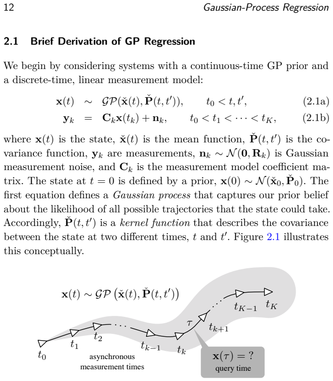
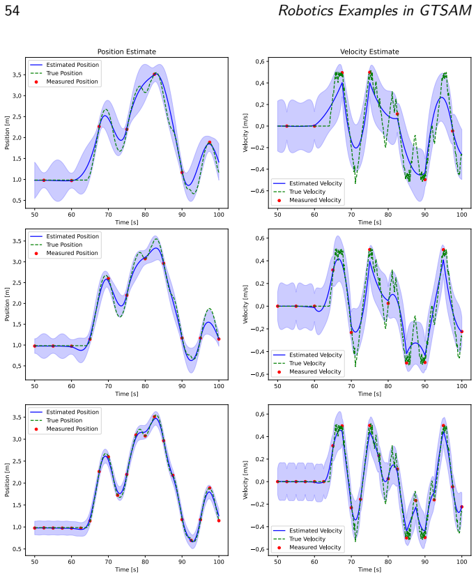
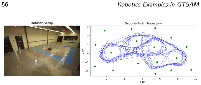
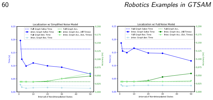
Continuous-time state estimation is gaining in popularity due to its abilities to provide smooth solutions, handle asynchronous sensors, and interpolate between data points. While there are two main paradigms, parametric (e.g., temporal basis functions, splines) and nonparametric (Gaussian processes), the latter has seen less adoption despite its technical advantages and relative ease of implementation. In this article, we seek to rectify this situation by providing a new simplified explanation of GP continuous-time estimation rooted in the language of factor graphs, which have become the de facto estimation paradigm in much of robotics. To simplify onboarding, we also provide three working examples implemented in the popular GTSAM estimation framework.
Editorial analysis
A structured set of objections, weighed in public.
Referee Report
Summary. The paper presents a factor-graph formulation of Gaussian process (GP) continuous-time state estimation. It argues that GP methods offer advantages including trajectory smoothness, support for asynchronous sensors, and natural interpolation, yet have seen limited adoption; the work provides a simplified explanation in factor-graph language together with three working GTSAM implementations to lower the barrier for practitioners already using such libraries.
Significance. If the formulation and examples are correct, the paper has moderate significance as a bridge between nonparametric continuous-time estimation and the dominant factor-graph paradigm in robotics. The concrete, working GTSAM code constitutes direct evidence of implementability and reproducibility, which strengthens the claim of relative ease of onboarding and could aid wider adoption among existing GTSAM users.
minor comments (3)
- Abstract: the assertion that GP methods possess 'relative ease of implementation' is stated without a brief supporting comparison to parametric alternatives (e.g., splines); adding one sentence would strengthen the motivation.
- The manuscript would benefit from a short table or bullet list in the examples section that summarizes the three GTSAM implementations by sensor type, state dimension, and key GP kernel used.
- Conclusion: the final paragraph could explicitly note any remaining limitations of the factor-graph GP formulation (e.g., kernel choice or scaling with trajectory length) to give readers a balanced view.
Simulated Author's Rebuttal
We thank the referee for the positive review and recommendation to accept. We are pleased that the contribution of recasting Gaussian-process continuous-time estimation in factor-graph language, together with the concrete GTSAM implementations, has been recognized as a useful bridge for practitioners.
Circularity Check
Explanatory reformulation of prior GP continuous-time methods into factor graphs, with concrete implementations
full rationale
The paper reformulates existing Gaussian-process motion priors using factor-graph language and supplies three working GTSAM examples to demonstrate onboarding ease. No derivation, prediction, or uniqueness claim reduces by construction to a parameter or result defined inside the present manuscript. Self-citations to foundational GP work (e.g., Barfoot et al.) provide background context but are not load-bearing for the central contribution, which rests on the supplied implementations rather than any closed mathematical loop. The work is self-contained as an expository bridge between estimation paradigms.
Axiom & Free-Parameter Ledger
axioms (2)
- domain assumption Gaussian processes provide a suitable nonparametric prior for continuous-time motion
- domain assumption Factor graphs are the de-facto estimation paradigm in robotics
Reference graph
Works this paper leans on
-
[1]
Dellaert, Frank and Kaess, Michael , year =. Factor. Foundations and Trends. doi:10.1561/2300000043 , urldate =
-
[2]
Dong, Jing and Mukadam, Mustafa and Boots, Byron and Dellaert, Frank , year =. Sparse. 2018. doi:10.1109/ICRA.2018.8461077 , urldate =
-
[3]
Johnson, Jacob C. and Mangelson, Joshua G. and Beard, Randal W. , year =. Continuous-. IEEE Robotics and Automation Letters , volume =. doi:10.1109/LRA.2022.3224364 , urldate =
-
[4]
The International Journal of Robotics Research , volume =
Kaess, Michael and Johannsson, Hordur and Roberts, Richard and Ila, Viorela and Leonard, John J and Dellaert, Frank , year =. The International Journal of Robotics Research , volume =. doi:10.1177/0278364911430419 , urldate =
-
[5]
Continuous Latent State Preintegration for Inertial-Aided Systems , author =. 2023 , month = sep, journal =. doi:10.1177/02783649231199537 , urldate =
-
[6]
Le Gentil, Cedric and. Gaussian. 2020 , month = apr, journal =. doi:10.1109/LRA.2020.2970940 , urldate =
-
[7]
Continuous-time gaussian process motion planning via probabilistic inference,
Mukadam, Mustafa and Dong, Jing and Yan, Xinyan and Dellaert, Frank and Boots, Byron , year =. Continuous-Time. The International Journal of Robotics Research , volume =. doi:10.1177/0278364918790369 , urldate =
-
[8]
Yan, Xinyan and Indelman, Vadim and Boots, Byron , year =. Incremental. doi:10.48550/arXiv.1504.02696 , urldate =. arXiv , keywords =:1504.02696 , primaryclass =
-
[9]
Yan, Xinyan and Indelman, Vadim and Boots, Byron , year =. Incremental Sparse. Robotics and Autonomous Systems , volume =. doi:10.1016/j.robot.2016.10.004 , urldate =
-
[10]
Lynch, Kevin M and Park, Frank C , date-added =. Modern robotics , year =
-
[11]
An introduction to optimization on smooth manifolds , year =
Boumal, Nicolas , date-added =. An introduction to optimization on smooth manifolds , year =
-
[12]
Factor graphs for robot perception , volume =
Dellaert, Frank and Kaess, Michael , date-added =. Factor graphs for robot perception , volume =. Foundations and Trends
-
[13]
A tutorial on se (3) transformation parameterizations and on-manifold optimization , volume =
Blanco, Jose-Luis , date-added =. A tutorial on se (3) transformation parameterizations and on-manifold optimization , volume =. University of Malaga, Tech. Rep , number =
-
[14]
Uncertainties in Galilean Spacetime , year =
Giefer, Lino Antoni , booktitle =. Uncertainties in Galilean Spacetime , year =. doi:10.23919/FUSION49465.2021.9627044 , keywords =
- [15]
-
[16]
Problema algebraicum ob affectiones prorsus singulares memorabile , volume =
Leonhard Euler , date-added =. Problema algebraicum ob affectiones prorsus singulares memorabile , volume =. Novi Commentarii Academiae Scientiarum Petropolitanae , note =
-
[17]
International Journal of Robotics Research (IJRR) , title =
S Lilge and T D Barfoot and J Burgner-Kahrs , date-added =. International Journal of Robotics Research (IJRR) , title =. 2022 , bdsk-file-1 =
work page 2022
-
[18]
A micro Lie theory for state estimation in robotics , year =
Sol. A micro Lie theory for state estimation in robotics , year =
-
[19]
The Bernoulli numbers: a brief primer , year =
Larson, Nathaniel , date-added =. The Bernoulli numbers: a brief primer , year =
-
[20]
On the exponential solution of differential equations for a linear operator , volume =
Magnus, Wilhelm , date-added =. On the exponential solution of differential equations for a linear operator , volume =. Communications on pure and applied mathematics , number =
-
[21]
The Magnus expansion and some of its applications , volume =
Blanes, Sergio and Casas, Fernando and Oteo, Jose-Angel and Ros, Jos. The Magnus expansion and some of its applications , volume =. Physics reports , number =
-
[22]
An online trajectory generator on SE (3) for human--robot collaboration , volume =
Huber, Gerold and Wollherr, Dirk , date-added =. An online trajectory generator on SE (3) for human--robot collaboration , volume =. Robotica , number =
-
[23]
A Goudar and W Zhao and T D Barfoot and A P Schoellig , booktitle =. Gaussian Variational Inference with Covariance Constraints Applied to Range-Only Localization , year =
-
[24]
Invariant kalman filtering , volume =
Barrau, Axel and Bonnabel, Silvere , date-added =. Invariant kalman filtering , volume =. Annual Review of Control, Robotics, and Autonomous Systems , pages =
-
[25]
The Invariant Extended Kalman Filter as a Stable Observer , volume =
Barrau, Axel and Bonnabel, Silv. The Invariant Extended Kalman Filter as a Stable Observer , volume =. IEEE Transactions on Automatic Control , number =. 2017 , bdsk-url-1 =
work page 2017
-
[26]
The vectorial parameterization of rotation , volume =
Bauchau, Olivier A and Trainelli, Lorenzo , date-added =. The vectorial parameterization of rotation , volume =. Nonlinear dynamics , number =
-
[27]
Vectorial Parameterizations of Pose , year =
T D Barfoot and J R Forbes and G M T D'Eleuterio , date-added =. Vectorial Parameterizations of Pose , year =. Robotica , note =
-
[28]
arXiv preprint arXiv:2102.07432 , title =
Ablin, Pierre and Peyr. arXiv preprint arXiv:2102.07432 , title =
-
[29]
Aided navigation: GPS with high rate sensors , year =
Farrell, Jay , date-added =. Aided navigation: GPS with high rate sensors , year =
-
[30]
Royal Society Proceedings A , title =
G M T D'Eleuterio and T D Barfoot , date-added =. Royal Society Proceedings A , title =
-
[31]
Computing integrals involving the matrix exponential , volume =
Van Loan, Charles , date-added =. Computing integrals involving the matrix exponential , volume =. IEEE transactions on automatic control , number =
-
[32]
Brossard, Martin and Barrau, Axel and Chauchat, Paul and Bonnabel, Silv. Associating uncertainty to extended poses for on lie group IMU preintegration with rotating Earth , year =. IEEE Transactions on Robotics , publisher =
-
[33]
Linear observation systems on groups (I) , year =
Barrau, Axel and Bonnabel, Silvere , date-added =. Linear observation systems on groups (I) , year =
-
[34]
Non-linear state error based extended Kalman filters with applications to navigation , year =
Barrau, Axel , date-added =. Non-linear state error based extended Kalman filters with applications to navigation , year =
-
[35]
Continuous Integration over SO(3) for IMU Preintegration , year =
Le Gentil, Cedric and Vidal-Calleja, Teresa , booktitle =. Continuous Integration over SO(3) for IMU Preintegration , year =
-
[36]
Forster, Christian and Carlone, Luca and Dellaert, Frank and Scaramuzza, Davide , booktitle =. IMU preintegration on manifold for efficient visual-inertial maximum-a-posteriori estimation , year =
-
[37]
Lupton, Todd and Sukkarieh, Salah , date-added =. Visual-inertial-aided navigation for high-dynamic motion in built environments without initial conditions , volume =. IEEE Transactions on Robotics , number =
-
[38]
A Data-Driven Motion Prior for Continuous-Time Trajectory Estimation on SE(3) , url =
J N Wong and D J Yoon and A P Schoellig and T D Barfoot , date-added =. A Data-Driven Motion Prior for Continuous-Time Trajectory Estimation on SE(3) , url =. 2020 , bdsk-file-1 =. doi:10.1109/LRA.2020.2969153 , journal =
-
[39]
A White-Noise-On-Jerk Motion Prior for Continuous-Time Trajectory Estimation on SE(3) , url =
T Y Tang and D J Yoon and T D Barfoot , date-added =. A White-Noise-On-Jerk Motion Prior for Continuous-Time Trajectory Estimation on SE(3) , url =. 2019 , bdsk-file-1 =. doi:10.1109/LRA.2019.2891492 , journal =
-
[40]
Batch Continuous-Time Trajectory Estimation , url =
S W Anderson , date-added =. Batch Continuous-Time Trajectory Estimation , url =. 2016 , bdsk-file-1 =
work page 2016
-
[41]
Symmetry-preserving observers , volume =
Bonnabel, Silvere and Martin, Philippe and Rouchon, Pierre , date-added =. Symmetry-preserving observers , volume =. IEEE Transactions on Automatic Control , number =
-
[42]
Equivariant filter design for kinematic systems on lie groups , volume =
Mahony, Robert and Trumpf, Jochen , date-added =. Equivariant filter design for kinematic systems on lie groups , volume =. IFAC-PapersOnLine , number =
-
[43]
The invariant extended Kalman filter as a stable observer , volume =
Barrau, Axel and Bonnabel, Silv. The invariant extended Kalman filter as a stable observer , volume =. IEEE Transactions on Automatic Control , number =
-
[44]
and Ghaffari, Maani and Vasudevan, Ram and Eustice, Ryan M
Mangelson, Joshua G. and Ghaffari, Maani and Vasudevan, Ram and Eustice, Ryan M. , date-added =. Characterizing the Uncertainty of Jointly Distributed Poses in the Lie Algebra , volume =. IEEE Transactions on Robotics , number =. 2020 , bdsk-url-1 =
work page 2020
-
[45]
Statistical Inference for Probabilistic Functions of Finite State Markov Chains , volume =
L Baum and T Petrie , date-added =. Statistical Inference for Probabilistic Functions of Finite State Markov Chains , volume =. Annals of Mathematical Statistics , number =
-
[46]
Approximating Discrete Probability Distributions With Dependence Trees , volume =
C K Chow and C N Liu , date-added =. Approximating Discrete Probability Distributions With Dependence Trees , volume =. IEEE Transactions on Information Theory , number =
-
[47]
Probabilistic Graphical Models: Principles and Techniques , year =
D Koller and N Friedman , date-added =. Probabilistic Graphical Models: Principles and Techniques , year =
-
[48]
An Approach to Time Series Smoothing and Forecasting Using the
R H Shumway and D S Stoffer , date-added =. An Approach to Time Series Smoothing and Forecasting Using the. Journal of Time Series Analysis , number =
-
[49]
Sur les fonctions convexes et les in
Jensen, Johan Ludwig William Valdemar , date-added =. Sur les fonctions convexes et les in. Acta mathematica , pages =
-
[50]
Cubature Kalman Filters , volume =
I Arasaratnam and S Haykin , date-added =. Cubature Kalman Filters , volume =. IEEE Transactions on Automatic Control , number =
-
[51]
Constructing Cubature Formulae: The Science Behind the Art , volume =
R Cools , date-added =. Constructing Cubature Formulae: The Science Behind the Art , volume =. Acta Numerica , pages =
-
[52]
Gaussian Filters for Nonlinear Filtering Problems , volume =
K Ito and K Xiong , date-added =. Gaussian Filters for Nonlinear Filtering Problems , volume =. IEEE Transactions on Automatic Control , number =
-
[53]
High-degree Cubature Kalman Filter , volume =
B Jia and M Xin and Y Cheng , date-added =. High-degree Cubature Kalman Filter , volume =. Automatica , pages =
-
[54]
Numerical Recipes: The Art of Scientific Computing , year =
W H Press and S A Teukolsky and W T Vetterling and B P Flannery , date-added =. Numerical Recipes: The Art of Scientific Computing , year =
-
[55]
Bayes--Hermite quadrature , volume =
O'Hagan, Anthony , date-added =. Bayes--Hermite quadrature , volume =. Journal of statistical planning and inference , number =
-
[56]
On the Relation Between Gaussian Process Quadratures and Sigma-Point Methods , volume =
S S\". On the Relation Between Gaussian Process Quadratures and Sigma-Point Methods , volume =. Journal of Advances in Information Fusion , number =
-
[57]
Fourier-Hermite Kalman Filter , volume =
J Sarmavuori and S S\". Fourier-Hermite Kalman Filter , volume =. IEEE Transactions on Automatic Control , number =
-
[58]
A Numerical-Integration Perspective on Gaussian Filters , volume =
Y Wu and D Hu and M Wu and X Hu , date-added =. A Numerical-Integration Perspective on Gaussian Filters , volume =. IEEE Transactions on Signal Processing , number =
-
[59]
On Computing Certain Elements of the Inverse of a Sparse Matrix , volume =
A M Erisman and W F Tinney , date-added =. On Computing Certain Elements of the Inverse of a Sparse Matrix , volume =. Commununications of the ACM , number =. 1975 , bdsk-url-1 =
work page 1975
-
[60]
Golub, HG and Van Loan, Charles F , date-added =. Press, London , title =
-
[61]
Broussolle, F , date-added =. State estimation in power systems: detecting bad data through the sparse inverse matrix method , year =. IEEE Transactions on Power Apparatus and Systems , number =
-
[62]
Covariance recovery from a square root information matrix for data association , volume =
Kaess, Michael and Dellaert, Frank , date-added =. Covariance recovery from a square root information matrix for data association , volume =. Robotics and autonomous systems , number =
-
[63]
A Review on the Inverse of Symmetric Tridiagonal and Block Tridiagonal Matrices , volume =
G Meurant , date-added =. A Review on the Inverse of Symmetric Tridiagonal and Block Tridiagonal Matrices , volume =. SIAM Journal of Matrix Analysis and Applications , number =
-
[64]
A Sparse Bus Impedance Matrix and its Application to Short Circuit Study , year =
K Takahashi and J Fagan and M-S Chen , booktitle =. A Sparse Bus Impedance Matrix and its Application to Short Circuit Study , year =
-
[65]
On the mathematical foundations of theoretical statistics , volume =
Fisher, Ronald A , date-added =. On the mathematical foundations of theoretical statistics , volume =. Philosophical Transactions of the Royal Society of London. Series A, Containing Papers of a Mathematical or Physical Character , number =
-
[66]
Natural gradient works efficiently in learning , volume =
Amari, Shun-Ichi , date-added =. Natural gradient works efficiently in learning , volume =. Neural computation , number =
-
[67]
Stochastic variational inference , volume =
Hoffman, Matthew D and Blei, David M and Wang, Chong and Paisley, John , date-added =. Stochastic variational inference , volume =. The Journal of Machine Learning Research , number =
-
[68]
Jordan and Zubin Ghahramani and Tommi Jaakkola and Lawrence K
Michael I. Jordan and Zubin Ghahramani and Tommi Jaakkola and Lawrence K. Saul , date-added =. An Introduction to Variational Methods for Graphical Models , volume =. Machine Learning , pages =
-
[69]
System identification of nonlinear state-space models , volume =
Sch. System identification of nonlinear state-space models , volume =. Automatica , number =
-
[70]
Parameter Estimation for Linear Dynamical Systems , year =
Z Ghahramani and G E Hinton , date-added =. Parameter Estimation for Linear Dynamical Systems , year =
-
[71]
Learning nonlinear dynamical systems using an EM algorithm , year =
Ghahramani, Zoubin and Roweis, Sam T , booktitle =. Learning nonlinear dynamical systems using an EM algorithm , year =
-
[72]
A view of the EM algorithm that justifies incremental, sparse, and other variants , year =
Neal, Radford M and Hinton, Geoffrey E , booktitle =. A view of the EM algorithm that justifies incremental, sparse, and other variants , year =
-
[73]
Application of unscented transformation in nonlinear system identification , volume =
Ga. Application of unscented transformation in nonlinear system identification , volume =. IFAC Proceedings Volumes , number =
-
[74]
Posterior linearization filter: Principles and implementation using sigma points , volume =
Garc. Posterior linearization filter: Principles and implementation using sigma points , volume =. IEEE transactions on signal processing , number =
-
[75]
Ala-Luhtala, Juha and S. Gaussian filtering and variational approximations for Bayesian smoothing in continuous-discrete stochastic dynamic systems , volume =. Signal Processing , month =. 2015 , bdsk-url-1 =
work page 2015
-
[76]
Expectation maximization based parameter estimation by sigma-point and particle smoothing , year =
Kokkala, Juho and Solin, Arno and S. Expectation maximization based parameter estimation by sigma-point and particle smoothing , year =. 17th International Conference on Information Fusion (FUSION) , date-added =
-
[77]
Kokkala, Juho and Solin, Arno and S. Sigma-point filtering and smoothing based parameter estimation in nonlinear dynamic systems , volume =. Journal of Advances in Information Fusion , number =
-
[78]
The variational Gaussian approximation revisited , volume =
Opper, Manfred and Archambeau, C. The variational Gaussian approximation revisited , volume =. Neural computation , number =
-
[79]
T D Barfoot and J R Forbes and D J Yoon , date-added =. Exactly Sparse Gaussian Variational Inference with Application to Derivative-Free Batch Nonlinear State Estimation , url =. 2020 , bdsk-file-1 =. doi:10.1177/0278364920937608 , journal =
-
[80]
Yang, Heng and Antonante, Pasquale and Tzoumas, Vasileios and Carlone, Luca , date-added =. Graduated non-convexity for robust spatial perception: From non-minimal solvers to global outlier rejection , volume =. IEEE Robotics and Automation Letters , number =
discussion (0)
Sign in with ORCID, Apple, or X to comment. Anyone can read and Pith papers without signing in.