arxiv: 2605.09500 · v2 · submitted 2026-05-10 · 🧮 math.NA · cs.NA· physics.comp-ph

Recognition: 2 theorem links

· Lean Theorem

A boundary integral method for wave scattering in a heterogeneous medium with a moving obstacle

Raaghav Ramani

Pith reviewed 2026-05-13 07:24 UTC · model grok-4.3

classification 🧮 math.NA cs.NAphysics.comp-ph

keywords boundary integral methodwave scatteringheterogeneous mediamoving obstaclesDoppler effectgeometric opticscausal geometrytime domain

0 comments

The pith

A time-domain boundary integral method formulates wave scattering in heterogeneous media with moving obstacles solely on the obstacle boundary.

A machine-rendered reading of the paper's core claim, the machinery that carries it, and where it could break.

The paper introduces a numerical technique for simulating linear waves that bend due to varying material properties and shift frequency from moving objects. Instead of discretizing the entire volume, the equations are reduced to integrals over just the surface of the moving obstacle. This is done by using a geometric-optics approximation to describe the main wave fronts and by tracking how the arrival times of signals are distorted by both the medium and the motion. The resulting method reproduces known effects such as waves wrapping around gas bubbles and Doppler shifts from a rotating turbine, remaining stable at speeds up to Mach 0.9.

Core claim

The central claim is that a geometric-optics parametrix combined with a ray-based description of the distorted causal geometry produces a well-posed boundary integral equation for the wave field that remains posed only on the worldsheet of the moving obstacle, thereby extending classical boundary-integral techniques from the homogeneous fixed-boundary case to the heterogeneous moving-boundary case.

What carries the argument

The combination of a geometric-optics parametrix for defining layer potentials and a ray-based characterization of the distorted causal geometry arising from the intersection of light cones with the moving boundary's worldsheet.

If this is right

The formulation avoids any volumetric mesh and therefore scales with surface area rather than volume.
Doppler shifts from obstacles moving at up to Mach 0.9 are resolved without artificial numerical dissipation.
Refractive focusing and defocusing produced by spherical inclusions are captured by the boundary operators alone.
The same framework handles both acoustic and electromagnetic waves once the appropriate fundamental solution is supplied.
Rotating or translating rigid bodies such as turbines can be treated by updating only the surface quadrature points at each time step.

Where Pith is reading between the lines

These are editorial extensions of the paper, not claims the author makes directly.

The same ray-tracking idea could be reused to derive boundary-only schemes for other hyperbolic systems such as Maxwell or elasticity equations with moving interfaces.
Because the method never discretizes the exterior, it may be particularly efficient for inverse problems that seek to recover moving-object trajectories from surface measurements.
Extending the geometric-optics parametrix to include higher-order transport corrections would allow the method to handle caustics without additional regularization.

Load-bearing premise

Leading wave behavior near fronts is accurately captured by geometric-optics rays and the causal structure of signal arrival can be completely determined by tracking those rays to their intersections with the moving boundary.

What would settle it

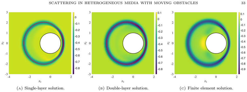
A side-by-side comparison of the boundary-integral solution against an independent high-resolution volumetric simulation or an exact solution for a simple case such as a sphere moving through a radially varying medium, checking whether predicted Doppler frequency shifts and refraction patterns match within discretization error.

Figures

Figures reproduced from arXiv: 2605.09500 by Raaghav Ramani.

**Figure 1.** Figure 1: Left: Two-dimensional schematic of the moving interface Γ(t) separating the interior domain Ω−(t) from the exterior domain Ω+(t), with outward normal velocity Un. Right: Smooth interior–exterior sound-speed contrast, in which the sound speed transitions across a thin interfacial layer Ωδ between the interior and exterior fields c−(x, t) and c +(x, t) in Ω−(t) and Ω+(t), respectively. Numerical methods for … view at source ↗

**Figure 2.** Figure 2: Geometry of wave propagation in a heterogeneous medium. The true cone consists of all spacetime points reachable from the source (y, τ) by signals propagating with local speed c(x, t), while the sourcefrozen cone assumes the constant emission speed c(y, τ). Left: True (blue) and source-frozen (red) cones in 2+1–space-time. The true cone is given by t − τ = η(x, t; y, τ), where η denotes the travel-time f… view at source ↗

**Figure 3.** Figure 3: Left: Backward light cone (blue surface) and worldsheet (red surface) plotted in 2+1 space-time. The purple curve is the intersection of the light cone with the worldsheet. Middle: Backward light cone emanating from (zk(α), tk) shown in a one-dimensional spatial slice. The blue shaded region represents the backward causal region, and the horizontal band indicates the current source time slab Tℓ = (tℓ−1, tℓ… view at source ↗

**Figure 4.** Figure 4: Element maps used in the P 1 discretization. Left: Reference element Eˆ. Middle: Image under the affine map αˆE onto E ⊂ S 2 . Right: Physical surface triangle ΓE(t) = z(E, t) on Γ(t). 4.3.2. P 1 approximation of boundary densities. We approximate the boundary densities σℓ(α) and µℓ(α), α ∈ S 2 , by continuous piecewise linear functions on Th. Let {αi} Nh i=1 ∈ T v h denote the mesh vertices. Define the no… view at source ↗

**Figure 5.** Figure 5: Fixed circle R(t) = 1 test. Left: Time history of the spatially averaged boundary density, comparing the numerical solutions σ∆ and µ∆ for N = 200 with the exact solution. Center: Numerical single-layer potential ϕ∆(x, t) obtained from the N = 200 solution at the final time. Right: Convergence of the error in the L2 xL2 t and L∞x L∞t norms for both single-layer and double-layer formulations. 5.1.2. Moving … view at source ↗

**Figure 6.** Figure 6: Expanding circle R(t) = 1 + U t test with U = 0.5. Left: Time history of the spatially averaged single-layer density σ∆ computed without stabilization, showing the onset of spurious oscillations and eventual instability. Center: Stabilized boundary densities σ∆ and µ∆ obtained using the Rynne timeaveraging procedure, which remain stable and in good agreement with the exact solution. Right: Numerical sing… view at source ↗

**Figure 7.** Figure 7: Numerical solutions for the four Doppler tests with Mach number U = 0.5. In each panel, the interface is shown as the gray surface and the reflected wavefront as the black curve. The scattered potential in the plane x2 = 0, localized near the wavefront, is also displayed. (a) Reflected wavefront comparison. (b) Reflected wavefronts at t = 5.0 [PITH_FULL_IMAGE:figures/full_fig_p024_7.png] view at source ↗

**Figure 8.** Figure 8: Comparison of the reflected wavefronts in the plane x2 = 0 for the four Doppler tests at Mach number U = 0.5. Left: reflected wavefronts at the comparison times used in [PITH_FULL_IMAGE:figures/full_fig_p024_8.png] view at source ↗

**Figure 9.** Figure 9: Scattered-potential sensor histories for the four Doppler tests at Mach number U = 0.5. Left: history at the fixed sensor (−2, 0, 0). Right: history at a co-moving sensor, initialized at (−2, 0, 0) and transported with the sphere. the scattered potential shifts downward and becomes more vertically elongated. Across the range of Mach numbers tested, the computed solutions remain stable, including in the lar… view at source ↗

**Figure 10.** Figure 10: Mach number U parameter study for the rising configuration. In each panel, the reflected wavefront and the slice of the local scattered potential in the plane x2 = 0 are displayed at the final time tmax = 2.5. 5.3. Numerical example: scattering by a smooth rotating turbine. We consider a two-dimensional example in which the sound speed is constant, c(x, t) ≡ 1, and the scatterer is a smooth turbine-shaped… view at source ↗

**Figure 11.** Figure 11: Numerical solutions for the smooth turbine test. The top row shows the fixed case with U = 0.0, and the bottom row shows the rotating case with U = 0.5. In each panel, the reflected wavefront is shown as the red curve, and the scattered potential is shown as the heatmap. The scattered potential is computed only in the causal region behind the reflected front. 6.1.1. Hamiltonian ray equations. The stationa… view at source ↗

**Figure 12.** Figure 12: displays the computed solution at the final time tmax = 3. The left panel shows the x2 = 0 slice of the sound-speed field, together with a representative family of three-dimensional rays emanating from the source point (−1, 0, 0) and terminating at a selection of target points on the interface. The right panel shows the corresponding approximate scattered field ϕ˜(x, t) defined by (3.8a), restricted to th… view at source ↗

**Figure 13.** Figure 13: Reference comparison for the spherical gas-bubble test at the final nondimensional time t = 3. The plots show the slice of the scattered field ϕ˜(x, t) in the plane x2 = 0, with the reflected wavefront in that plane overlaid in red. Left: ambient reference case, obtained by setting c(x) ≡ C+ = 1. Right: gas-bubble case with the travel-time function approximated by the chord model (6.6). that the asymmetri… view at source ↗

**Figure 14.** Figure 14: Comparison at tmax = 3.0 for the benchmark problem with time-dependent sound speed (7.4)– (7.6). Left: two-dimensional single-layer solution with the reflected wavefront (red curve) overlaid. Middle: two-dimensional double-layer solution with the reflected wavefront (red curve) overlaid. Right: finite element solution of the same exterior scattering problem. In each panel, the obstacle boundary is shown … view at source ↗

**Figure 15.** Figure 15: Representative snapshots of the rising-fireball simulation at two selected times. In each panel, the fireball interface Γ(t) is shown as the triangulated gray surface. The computed reflected wavefront is shown as the translucent red surface, and its intersection with the plane x2 = 0 is shown as the black curve. Also displayed is the approximate scattered potential ϕ˜(x, t), defined in (3.8a), restricted … view at source ↗

**Figure 16.** Figure 16: Comparison between the hot-fireball simulation and the ambient-air reference case. Left: latetime snapshot of the ambient-air reference case, shown in the same style as [PITH_FULL_IMAGE:figures/full_fig_p035_16.png] view at source ↗

read the original abstract

We propose a time-domain boundary integral method to model linear wave propagation with refractive, focusing, and Doppler effects arising from medium heterogeneities and moving obstacles. In contrast to existing techniques, our method avoids volumetric discretization and yields a formulation posed only on the boundary of the obstacle. We combine two classical ingredients: a geometric--optics parametrix to capture leading-order behavior at propagating wavefronts, and a ray-based characterization of the distorted causal geometry. The former provides a framework for defining layer potentials and deriving the associated boundary integral equations, while the latter enables a pure boundary-only formulation. Taken together, these ingredients extend existing numerical techniques for the homogeneous, fixed-boundary case to the heterogeneous, moving-boundary setting, with appropriate modifications to capture the discrete causal structure arising from the intersection of distorted light cones with the worldsheet of the moving boundary. Numerical experiments demonstrate the ability of the method to resolve Doppler effects from moving obstacles, including a rotating turbine configuration, with stable performance up to Mach 0.9. In heterogeneous media, the method captures strong refractive effects from spherical inclusions: wave propagation wrapping around a gas bubble in water, and defocusing from a hot fireball rising through a stratified atmosphere.

Editorial analysis

A structured set of objections, weighed in public.

Desk editor's note, referee report, simulated authors' rebuttal, and a circularity audit. Tearing a paper down is the easy half of reading it; the pith above is the substance, this is the friction.

Desk Editor's Note private letter to a colleague

The paper gives a boundary-only time-domain integral method for waves in heterogeneous media with moving obstacles by combining a geometric-optics parametrix with ray tracing of the distorted causal geometry.

read the letter

The core advance is keeping everything on the obstacle boundary even when the background speed varies and the boundary itself moves. They achieve this by using the parametrix to handle the leading singular behavior of the fundamental solution and then using rays to track how the light cones intersect the worldsheet of the moving boundary. That lets them write layer potentials and the resulting integral equation without volume terms, which is the usual sticking point in these problems. The numerical examples back this up in practice: the rotating turbine at Mach 0.9 runs stably and shows the expected Doppler shift, while the spherical inclusion and stratified atmosphere cases capture refraction and defocusing without obvious artifacts. The discretization respects the discrete causal intersections, which is the necessary adjustment from the fixed homogeneous setting. The derivation stays consistent with classical boundary-integral theory, treating the parametrix only for the singular part and the integral operator for the regular remainder. The main limitation is that the abstract and stress-test note do not include explicit error estimates or convergence rates, so it is not yet clear how the accuracy scales with mesh size or time step in the general case. A few direct comparisons against a volumetric solver on the same test problems would also strengthen the claims. This work is aimed at researchers who already use boundary integral methods for time-domain acoustics or electromagnetics and need to add heterogeneity or motion without switching to volume methods. It is worth sending to a serious referee because the central construction is new, the numerical evidence is positive, and the approach addresses a practical gap even if further analysis is needed.

Referee Report

2 major / 2 minor

Summary. The manuscript proposes a time-domain boundary integral method for linear wave scattering in heterogeneous media containing moving obstacles. The approach combines a geometric-optics parametrix for leading-order wavefront behavior with a ray-based description of the distorted causal structure to derive a boundary integral equation posed solely on the worldsheet of the moving obstacle. Numerical experiments illustrate the method's ability to capture Doppler effects for a rotating turbine at Mach 0.9 and refractive phenomena such as wave wrapping around a gas bubble and defocusing in a stratified atmosphere.

Significance. Should the central formulation prove exact and the discretization convergent, the work would represent a notable advance in computational wave propagation by eliminating the need for volumetric discretization in complex heterogeneous and moving-boundary settings. This could enable efficient simulations in applications involving high-speed objects and varying media, with the reported stability at Mach 0.9 indicating potential for practical use in aeroacoustics and similar fields. The avoidance of volumetric meshes is a key strength if the boundary-only property holds rigorously.

major comments (2)

The derivation of the boundary integral equation using the parametrix is central but lacks explicit verification that the resulting operator is equivalent to the original PDE problem. Specifically, it is unclear how the regular part of the solution is recovered exactly from the integral equation without additional volume terms in the heterogeneous case.
While stability is reported up to Mach 0.9 for the turbine example, there is no convergence study or error analysis with respect to discretization parameters. This makes it difficult to assess the accuracy of the captured Doppler and refractive effects beyond visual inspection.

minor comments (2)

The phrase 'stable performance' should be quantified, e.g., by specifying the time-stepping scheme's CFL condition or observed growth rates.
Ensure that foundational works on geometric-optics parametrices for wave equations in heterogeneous media are cited to contextualize the contribution.

Simulated Author's Rebuttal

2 responses · 0 unresolved

We thank the referee for the thoughtful review and positive assessment of the manuscript's potential significance. We address the major comments point by point below, indicating where revisions will be made to strengthen the presentation.

read point-by-point responses

Referee: The derivation of the boundary integral equation using the parametrix is central but lacks explicit verification that the resulting operator is equivalent to the original PDE problem. Specifically, it is unclear how the regular part of the solution is recovered exactly from the integral equation without additional volume terms in the heterogeneous case.

Authors: The geometric-optics parametrix is constructed to satisfy the heterogeneous wave equation to leading order, with the remainder being smoother. The ray-based causal geometry then allows us to define retarded potentials that incorporate the medium heterogeneities without requiring explicit volume integrals. The boundary integral equation is derived by enforcing the boundary conditions on the worldsheet, and the equivalence follows from the properties of the parametrix and the fundamental solution in the heterogeneous medium. To make this more explicit, we will add a dedicated paragraph or subsection in the revised manuscript that verifies the recovery of the regular part by showing that the integral representation satisfies the PDE in the exterior domain. revision: yes
Referee: While stability is reported up to Mach 0.9 for the turbine example, there is no convergence study or error analysis with respect to discretization parameters. This makes it difficult to assess the accuracy of the captured Doppler and refractive effects beyond visual inspection.

Authors: We acknowledge that the current numerical section relies primarily on visual comparison with expected physical phenomena. In the revised manuscript, we will include a convergence study for the rotating turbine example, examining the error in the computed Doppler shift and pressure fields as the discretization parameters (number of boundary elements and time steps) are refined. This will provide quantitative evidence of the method's accuracy. revision: yes

Circularity Check

0 steps flagged

No significant circularity

full rationale

The derivation relies on two explicitly classical ingredients—a geometric-optics parametrix for leading singular behavior and a ray-based description of the distorted causal geometry—combined with standard layer-potential constructions for the boundary integral equation. These are presented as extensions of existing homogeneous fixed-boundary techniques rather than self-derived quantities. No parameter is fitted to data and then relabeled as a prediction, no uniqueness theorem is imported from the authors’ prior work, and the central claim (a pure boundary-only formulation) is obtained by enforcing the correct retarded potentials on the worldsheet, which is a direct consequence of the classical parametrix plus the ray geometry rather than a definitional tautology. The numerical examples serve only as validation, not as inputs to the derivation itself. The manuscript therefore remains self-contained against external benchmarks with no load-bearing step that reduces to its own inputs by construction.

Axiom & Free-Parameter Ledger

0 free parameters · 1 axioms · 0 invented entities

The approach relies on standard assumptions of linear wave propagation without introducing new free parameters or invented entities in the abstract.

axioms (1)

domain assumption Linear wave propagation governed by the wave equation holds in heterogeneous media.
Core modeling assumption enabling the boundary integral setup.

pith-pipeline@v0.9.0 · 5511 in / 1171 out tokens · 64801 ms · 2026-05-13T07:24:59.163725+00:00 · methodology

Review history (2 revisions) →

discussion (0)

Lean theorems connected to this paper

Citations machine-checked in the Pith Canon. Every link opens the source theorem in the public Lean library.

IndisputableMonolith/Foundation/RealityFromDistinction.lean reality_from_one_distinction unclear
We combine two classical ingredients: a geometric–optics parametrix to capture leading-order behavior at propagating wavefronts, and a ray-based characterization of the distorted causal geometry... G ≈ A G0(η, θ) where η solves the travel-time eikonal equation

Reference graph

Works this paper leans on

73 extracted references · 73 canonical work pages

[1]

Abboud, P

T. Abboud, P. Joly, J. Rodrı, I. Terrasse, et al.Coupling discontinuous Galerkin methods and retarded potentials for transient wave propagation on unbounded domains. Journal of Computational Physics, 230(15):5877–5907, 2011

work page 2011
[2]

R. S. Arthur, K. A. Lundquist, J. D. Mirocha, S. Neuscamman, Y. Kanarska, and J. S. Nasstrom. Simulating nuclear cloud rise within a realistic atmosphere using the Weather Research and Forecasting model. Atmospheric Environment, 254:118363, 2021

work page 2021
[3]

T. G. Ayele, B. M. Demissie, and S. E. Mikhailov.Boundary-Domain Integral Equations for Variable- Coefficient Helmholtz BVPs in 2D. Journal of Mathematical Sciences, 280(3):330–355, 2024

work page 2024
[4]

Banjai and S

L. Banjai and S. Sauter.Rapid solution of the wave equation in unbounded domains. SIAM Journal on Numerical Analysis, 47(1):227–249, 2009

work page 2009
[5]

Banjai, C

L. Banjai, C. Lubich, and F.-J. Sayas.Stable numerical coupling of exterior and interior problems for the wave equation. Numerische Mathematik, 129(4):611–646, 2015

work page 2015
[6]

Berenger.A perfectly matched layer for the absorption of electromagnetic waves

J.-P. Berenger.A perfectly matched layer for the absorption of electromagnetic waves. Journal of computational physics, 114(2):185–200, 1994

work page 1994
[7]

K. S. Brentner and F. Farassat.Analytical comparison of the acoustic analogy and Kirchhoff formulation for moving surfaces. AIAA journal, 36(8):1379–1386, 1998

work page 1998
[8]

O. P. Bruno and E. M. Hyde.Higher-order Fourier approximation in scattering by two-dimensional, inhomogeneous media. SIAM Journal on Numerical Analysis, 42(6):2298–2319, 2005. SCATTERING IN HETEROGENEOUS MEDIA WITH MOVING OBSTACLES 43

work page 2005
[9]

O. P. Bruno and L. A. Kunyansky.A fast, high-order algorithm for the solution of surface scattering problems: basic implementation, tests, and applications. Journal of Computational Physics, 169(1): 80–110, 2001

work page 2001
[10]

S. N. Chandler-Wilde, I. G. Graham, S. Langdon, and E. A. Spence.Numerical-asymptotic boundary integral methods in high-frequency acoustic scattering. Acta Numerica, 21:89–305, 2012

work page 2012
[11]

D. L. Colton, R. Kress, and R. Kress.Inverse acoustic and electromagnetic scattering theory, volume 93. Springer, 1998

work page 1998
[12]

Cooper.Scattering of plane waves by a moving obstacle

J. Cooper.Scattering of plane waves by a moving obstacle. Archive for Rational Mechanics and Analysis, 71(2):113–141, 1979

work page 1979
[13]

Cooper and W

J. Cooper and W. Strauss.Representations of the scattering operator for moving obstacles. Indiana University Mathematics Journal, 28(4):643–671, 1979

work page 1979
[14]

Cooper and W

J. Cooper and W. Strauss.The leading singularity of a wave reflected by a moving boundary. Journal of Differential Equations, 52(2):175–203, 1984

work page 1984
[15]

Costabel and F.-J

M. Costabel and F.-J. Sayas.Time-dependent problems with the boundary integral equation method. Encyclopedia of computational mechanics, 1:703–721, 2004

work page 2004
[16]

Costabel and E

M. Costabel and E. Stephan.A direct boundary integral equation method for transmission problems. Journal of mathematical analysis and applications, 106(2):367–413, 1985

work page 1985
[17]

P. J. Davies and D. B. Duncan.Averaging techniques for time-marching schemes for retarded potential integral equations. Applied Numerical Mathematics, 23(3):291–310, 1997

work page 1997
[18]

The journal of the acoustical society of America, 100(1):98–107, 1996

L.DeLacerda, L.Wrobel, andW.Mansur.A boundary integral formulation for two-dimensional acoustic radiation in a subsonic uniform flow. The journal of the acoustical society of America, 100(1):98–107, 1996

work page 1996
[19]

De Rubeis, M

B. De Rubeis, M. Gennaretti, C. Poggi, and G. Bernardini.Sound Scattered by Deforming Bodies Through Boundary Integral Formulations. AIAA Journal, 63(10):4196–4209, 2025

work page 2025
[20]

Dominguez, M

V. Dominguez, M. Ganesh, and F.-J. Sayas.An overlapping decomposition framework for wave propaga- tion in heterogeneous and unbounded media: Formulation, analysis, algorithm, and simulation. Journal of Computational Physics, 403:109052, 2020

work page 2020
[21]

Engquist and A

B. Engquist and A. Majda.Absorbing boundary conditions for the numerical simulation of waves. Mathematics of computation, 31(139):629–651, 1977

work page 1977
[22]

Engquist and O

B. Engquist and O. Runborg.Computational high frequency wave propagation. Acta numerica, 12: 181–266, 2003

work page 2003
[23]

A. A. Ergin, B. Shanker, and E. Michielssen.Fast evaluation of three-dimensional transient wave fields using diagonal translation operators. Journal of Computational Physics, 146(1):157–180, 1998

work page 1998
[24]

Eskin.Lectures on linear partial differential equations, volume 123

G. Eskin.Lectures on linear partial differential equations, volume 123. American Mathematical Soc., 2011

work page 2011
[25]

J. E. Ffowcs Williams and D. L. Hawkings.Sound generation by turbulence and surfaces in arbitrary motion. Philosophical Transactions of the Royal Society of London. Series A, Mathematical and Physical Sciences, 264(1151):321–342, 1969

work page 1969
[26]

French and T

D. French and T. Peterson.A continuous space-time finite element method for the wave equation. Mathematics of Computation, 65(214):491–506, 1996

work page 1996
[27]

F. G. Friedlander.The wave equation on a curved space-time, volume 2. Cambridge university press, 1975

work page 1975
[28]

Ganesh and I

M. Ganesh and I. G. Graham.A high-order algorithm for obstacle scattering in three dimensions. Journal of Computational Physics, 198(1):211–242, 2004

work page 2004
[29]

Ganesh, I

M. Ganesh, I. Graham, and J. Sivaloganathan.A new spectral boundary integral collocation method for three-dimensional potential problems. SIAM journal on numerical analysis, 35(2):778–805, 1998

work page 1998
[30]

Gennaretti, B

M. Gennaretti, B. De Rubeis, C. Poggi, and G. Bernardini.Deformable-boundary integral formulation for the solution of arbitrarily-forced acoustic wave equation. Journal of Sound and Vibration, 591:118618, 2024

work page 2024
[31]

Gimbutas and S

Z. Gimbutas and S. Veerapaneni.A fast algorithm for spherical grid rotations and its application to singular quadrature. SIAM Journal on Scientific Computing, 35(6):A2738–A2751, 2013

work page 2013
[32]

M. J. Grote, A. Schneebeli, and D. Schötzau.Discontinuous Galerkin finite element method for the wave equation. SIAM Journal on Numerical Analysis, 44(6):2408–2431, 2006. 44 RAAGHA V RAMANI

work page 2006
[33]

Ha-Duong.On retarded potential boundary integral equations and their discretisation

T. Ha-Duong.On retarded potential boundary integral equations and their discretisation. InTopics in Computational Wave Propagation: Direct and Inverse Problems, pages 301–336. Springer, 2003

work page 2003
[34]

Ha-Duong, A

T. Ha-Duong, A. Bamberger, and J. Nedelec.Formulation variationnelle espace-temps pour le calcul par potentiel retardé de la diffraction d’une onde acoustique (I). Mathematical methods in the applied sciences, 8(1):405–435, 1986

work page 1986
[35]

Ha-Duong, B

T. Ha-Duong, B. Ludwig, and I. Terrasse.A Galerkin BEM for transient acoustic scattering by an absorbing obstacle. International Journal for Numerical Methods in Engineering, 57(13):1845–1882, 2003

work page 2003
[36]

Hörmander.The analysis of linear partial differential operators III: Pseudo-differential operators

L. Hörmander.The analysis of linear partial differential operators III: Pseudo-differential operators. Springer Science & Business Media, 2007

work page 2007
[37]

F. Q. Hu, M. E. Pizzo, and D. M. Nark.On a time domain boundary integral equation formulation for acoustic scattering by rigid bodies in uniform mean flow. The Journal of the Acoustical Society of America, 142(6):3624–3636, 2017

work page 2017
[38]

J. B. Keller.Geometrical Theory of Diffraction. J. Opt. Soc. Am., 52(2):116–130, Feb 1962

work page 1962
[39]

Klöckner, A

A. Klöckner, A. Barnett, L. Greengard, and M. O’Neil.Quadrature by expansion: A new method for the evaluation of layer potentials. Journal of Computational Physics, 252:332–349, 2013

work page 2013
[40]

I. A. Kravtsov and Y. I. Orlov.Geometrical optics of inhomogeneous media, volume 38. Springer, 1990

work page 1990
[41]

A. R. Laliena and F.-J. Sayas.Theoretical aspects of the application of convolution quadrature to scattering of acoustic waves. Numerische Mathematik, 112(4):637–678, 2009

work page 2009
[42]

P. D. Lax.Asymptotic solutions of oscillatory initial value problems. Duke Mathematical Journal, 24 (4):627 – 646, 1957

work page 1957
[43]

J.-F. Lee, R. Lee, and A. Cangellaris.Time-domain finite-element methods. IEEE transactions on antennas and propagation, 45(3):430–442, 1997

work page 1997
[44]

Lombard and J

B. Lombard and J. Piraux.Numerical treatment of two-dimensional interfaces for acoustic and elastic waves. Journal of Computational Physics, 195(1):90–116, 2004

work page 2004
[45]

W. Lu, Y. Y. Lu, and J. Qian.Perfectly matched layer boundary integral equation method for wave scattering in a layered medium. SIAM Journal on Applied Mathematics, 78(1):246–265, 2018

work page 2018
[46]

W. J. Mansur.A time-stepping technique to solve wave propagation problems using the boundary element method. PhD thesis, University of Southampton, 1983

work page 1983
[47]

W. J. Mansur and C. Brebbia.Numerical implementation of the boundary element method for two dimensional transient scalar wave propagation problems. Applied Mathematical Modelling, 6(4):299– 306, 1982

work page 1982
[48]

P. A. Martin.Acoustic scattering by inhomogeneous obstacles. SIAM Journal on Applied Mathematics, 64(1):297–308, 2003

work page 2003
[49]

V. E. Ostashev and D. K. Wilson.Acoustics in moving inhomogeneous media. E & FN Spon London, 1997

work page 1997
[50]

C. S. Peskin.Flow patterns around heart valves: a numerical method. Journal of computational physics, 10(2):252–271, 1972

work page 1972
[51]

Ramani and S

R. Ramani and S. Shkoller.A multiscale model for Rayleigh-Taylor and Richtmyer-Meshkov instabilities. Journal of Computational Physics, 405:109177, 2020

work page 2020
[52]

S. Rao, D. Wilton, and A. Glisson.Electromagnetic scattering by surfaces of arbitrary shape. IEEE Transactions on antennas and propagation, 30(3):409–418, 1982

work page 1982
[53]

Rieder, F.-J

A. Rieder, F.-J. Sayas, and J. Melenk.Time domain boundary integral equations and convolution quadrature for scattering by composite media. Mathematics of Computation, 91(337):2165–2195, 2022

work page 2022
[54]

Rokhlin.Rapid solution of integral equations of scattering theory in two dimensions

V. Rokhlin.Rapid solution of integral equations of scattering theory in two dimensions. Journal of Computational physics, 86(2):414–439, 1990

work page 1990
[55]

Rynne and P

B. Rynne and P. Smith.Stability of time marching algorithms for the electric field integral equation. Journal of electromagnetic waves and applications, 4(12):1181–1205, 1990

work page 1990
[56]

Sambridge and B

M. Sambridge and B. Kennett.Boundary value ray tracing in a heterogeneous medium: a simple and versatile algorithm. Geophysical Journal International, 101(1):157–168, 1990

work page 1990
[57]

S. A. Sauter and C. Schwab.Boundary element methods. InBoundary Element Methods, pages 183–287. Springer, 2010

work page 2010
[58]

Sayas.Retarded Potentials and Time Domain Boundary Integral Equations

F.-J. Sayas.Retarded Potentials and Time Domain Boundary Integral Equations. Springer, 2013. SCATTERING IN HETEROGENEOUS MEDIA WITH MOVING OBSTACLES 45

work page 2013
[59]

Schädle, M

A. Schädle, M. López-Fernández, and C. Lubich.Fast and oblivious convolution quadrature. SIAM Journal on Scientific Computing, 28(2):421–438, 2006

work page 2006
[60]

J. H. Seo and R. Mittal.A high-order immersed boundary method for acoustic wave scattering and low-Mach number flow-induced sound in complex geometries. Journal of computational physics, 230(4): 1000–1019, 2011

work page 2011
[61]

J. A. Sethian.A fast marching level set method for monotonically advancing fronts.proceedings of the National Academy of Sciences, 93(4):1591–1595, 1996

work page 1996
[62]

Steinbach.Numerical approximation methods for elliptic boundary value problems: finite and bound- ary elements

O. Steinbach.Numerical approximation methods for elliptic boundary value problems: finite and bound- ary elements. Springer, 2008

work page 2008
[63]

W. A. Strauss.The existence of the scattering operator for moving obstacles. Journal of Functional Analysis, 31(2):255–262, 1979

work page 1979
[64]

Taflove.Review of the formulation and applications of the finite-difference time-domain method for numerical modeling of electromagnetic wave interactions with arbitrary structures

A. Taflove.Review of the formulation and applications of the finite-difference time-domain method for numerical modeling of electromagnetic wave interactions with arbitrary structures. Wave motion, 10(6): 547–582, 1988

work page 1988
[65]

Taflove, S

A. Taflove, S. C. Hagness, and M. Piket-May.Computational electromagnetics: the finite-difference time-domain method. The Electrical Engineering Handbook, 3(629-670):15, 2005

work page 2005
[66]

Um and C

J. Um and C. Thurber.A fast algorithm for two-point seismic ray tracing. Bulletin of the Seismological Society of America, 77(3):972–986, 1987

work page 1987
[67]

Vainikko.Fast solvers of the Lippmann-Schwinger equation

G. Vainikko.Fast solvers of the Lippmann-Schwinger equation. InDirect and inverse problems of mathematical physics, pages 423–440. Springer, 2000

work page 2000
[68]

Vinje, E

V. Vinje, E. Iversen, and H. Gjoystdal.Traveltime and amplitude estimation using wavefront construc- tion. Geophysics, 58(8):1157–1166, 1993

work page 1993
[69]

Wu and L

T. Wu and L. Lee.A direct boundary integral formulation for acoustic radiation in a subsonic uniform flow. Journal of sound and vibration, 175(1):51–63, 1994

work page 1994
[70]

L. Xia, H. Yuan, B. Wang, and W. Cai.Fast boundary integral method for acoustic wave scattering in two-dimensional layered media. arXiv preprint arXiv:2511.12450, 2025

work page arXiv 2025
[71]

G. Yu, W. Mansur, J. Carrer, and L. Gong.Stability of Galerkin and collocation time domain boundary element methods as applied to the scalar wave equation. Computers & Structures, 74(4):495–506, 2000

work page 2000
[72]

Zhang and R

C. Zhang and R. J. LeVeque.The immersed interface method for acoustic wave equations with discon- tinuous coefficients. Wave motion, 25(3):237–263, 1997

work page 1997
[73]

Zhao.A fast sweeping method for eikonal equations

H. Zhao.A fast sweeping method for eikonal equations. Mathematics of computation, 74(250):603–627, 2005. Center for Nonlinear Studies, Los Alamos National Laboratory, Los Alamos, NM 87545 Email address:rramani@lanl.gov

work page 2005