Recognition: 2 theorem links
· Lean TheoremRare transitions between collective states in an active fluid via a weakly nonlinear reduction
Pith reviewed 2026-05-12 02:34 UTC · model grok-4.3
The pith
Weakly nonlinear reduction of a noisy active fluid accurately predicts rare transitions between coexisting collective states.
A machine-rendered reading of the paper's core claim, the machinery that carries it, and where it could break.
Core claim
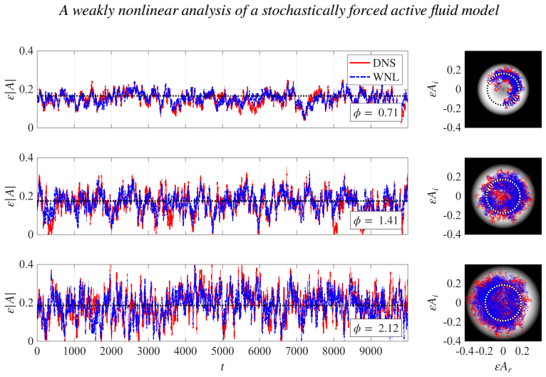
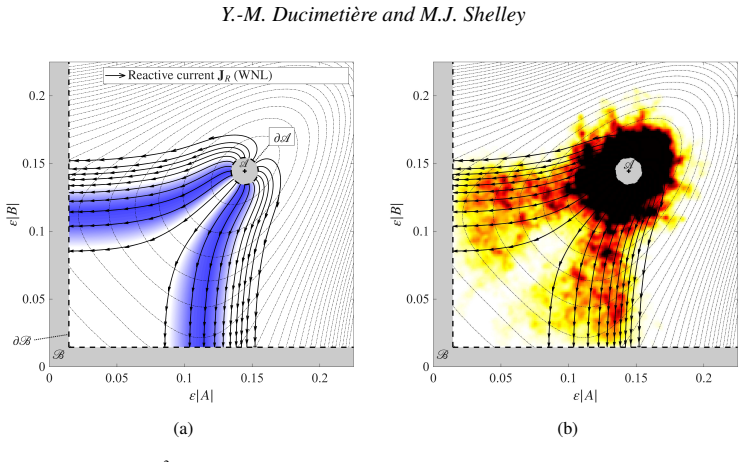
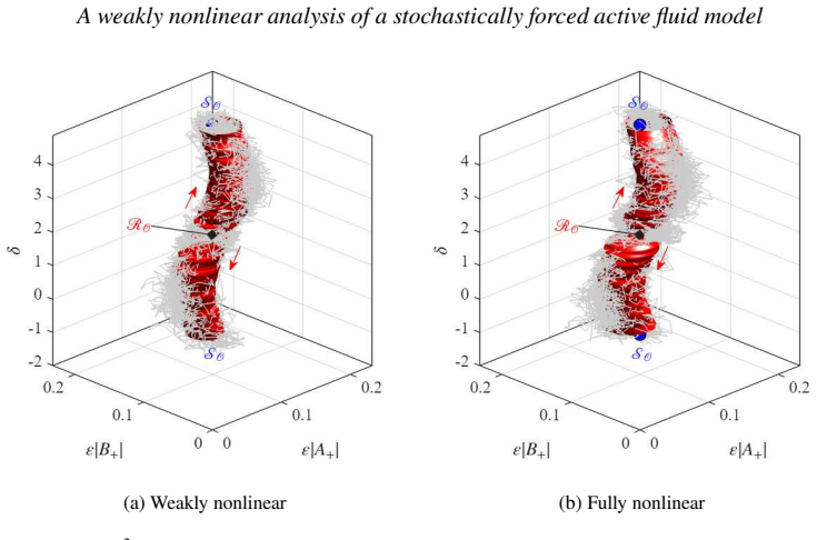
Past the onset of a codimension-4 Hopf bifurcation, the reduced stochastic amplitude equations exhibit two coexisting stable periodic orbits whose noise-induced transitions have mean times and out-of-equilibrium paths that agree quantitatively with those measured in the full stochastic PDE system, while being obtained at far lower computational cost.
What carries the argument
The stochastic amplitude equations obtained from the weakly nonlinear reduction, with noise terms derived analytically from the original spatio-temporal white noise.
If this is right
- Transition statistics can be extracted directly from the Fokker-Planck equation on the low-dimensional system.
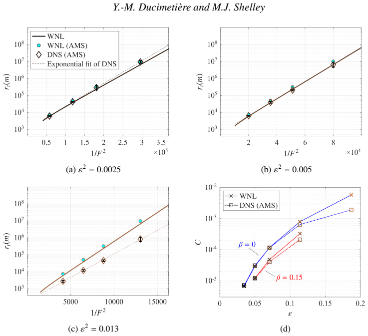
- The Adaptive Multilevel Splitting algorithm applied to the amplitude equations yields extremely long mean transition times between the two periodic orbits.
- The geometry of transition paths is explained by the invariant manifolds of the reduced system.
- The reduced model reproduces full-system statistics at considerably lower numerical cost.
Where Pith is reading between the lines
- The quantitative match implies that the essential mechanism of rare transitions is already encoded in the low-dimensional dynamics even away from the linear threshold.
- The same reduction procedure could be used to analyze noise-driven switching between collective states in other dilute active suspensions whose instabilities are captured by a weakly nonlinear expansion.
Load-bearing premise
The weakly nonlinear expansion and its derived stochastic terms remain accurate for rare-transition statistics even when the system is operated far from the bifurcation onset.
What would settle it
Full nonlinear simulations far below the critical diffusivity would show mean transition times or transition paths that deviate substantially from those computed on the reduced amplitude equations.
Figures


read the original abstract
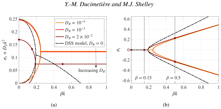
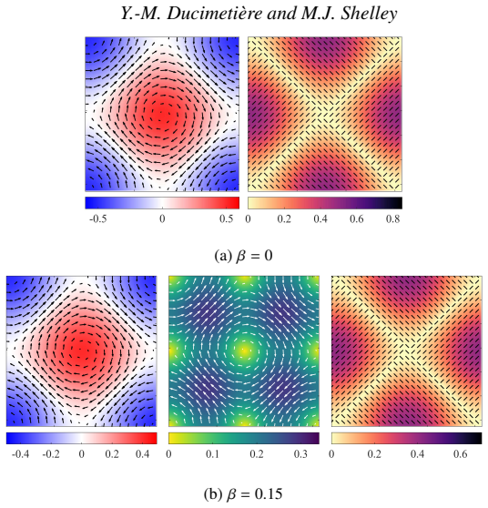
We study a model for a dilute suspension of rod-like particles swimming at constant velocity in a Stokes flow. As the translational diffusivity of the particles decreases, a two-dimensional uniform concentration of randomly aligned particles undergoes either a codimension-2 pitchfork bifurcation or a codimension-4 Hopf bifurcation, depending on the particles' swimming speed. We use a weakly nonlinear expansion to reduce the system to a low-dimensional one for the amplitudes of the bifurcating eigenmodes. The originality of our calculations lies in incorporating spatio-temporal white noise forcing. The stochastic forcing terms in the amplitude equations are derived analytically from the noise acting on the original system. Past the onset of the bifurcations, the particles deterministically self-organize into steady or oscillating states of collective motion. For the Hopf bifurcation scenario, two stable periodic orbits are found to coexist, each corresponding to a distinct collective dynamics. The stochastic forcing induces rare transitions between them. Owing to the low dimensionality of amplitude equations, steady and dynamical statistics can be computed directly from the Fokker-Planck equation, or via the Adaptive Multilevel Splitting (AMS) rare-event algorithm. In particular, extremely long mean transition times and associated out-of-equilibrium paths between the periodic orbits are obtained. These paths can be understood in light of the invariant manifolds of the low-dimensional system, which brings insights into the mechanism behind the transitions. We also performed fully nonlinear stochastic simulations and used the AMS algorithm directly on the full system. The statistics are in good quantitative agreement with those computed on the reduced systems, the latter being obtained at a considerably lower numerical cost.
Editorial analysis
A structured set of objections, weighed in public.
Referee Report
Summary. The manuscript analyzes a stochastic PDE model for a dilute suspension of rod-like particles swimming at constant speed in Stokes flow. As translational diffusivity decreases, the uniform isotropic state undergoes either a codimension-2 pitchfork or codimension-4 Hopf bifurcation depending on swimming speed. A weakly nonlinear expansion is used to derive stochastic amplitude equations, with the noise terms obtained analytically by projecting the spatio-temporal white noise onto the critical modes. In the Hopf case, two stable periodic orbits coexist; stochastic forcing induces rare transitions between them. Transition statistics (mean times and paths) are computed efficiently from the Fokker-Planck equation or via the Adaptive Multilevel Splitting algorithm on the reduced system and shown to agree quantitatively with direct AMS simulations of the full nonlinear stochastic PDE, at substantially lower cost. Transition mechanisms are interpreted through the invariant manifolds of the low-dimensional system.
Significance. If the reduced stochastic model remains faithful for the O(1) amplitude excursions that occur during rare transitions, the work supplies an analytically grounded, computationally efficient route to long-time statistics and mechanistic understanding of multistability in active fluids. The explicit derivation of the stochastic forcing terms from the original PDE and the side-by-side comparison with full-system simulations are clear strengths that distinguish the contribution from purely phenomenological reductions.
major comments (2)
- [Abstract] Abstract: the claim of 'good quantitative agreement' between AMS statistics of the reduced and full systems is presented without error bars, confidence intervals, or the specific distance from the codimension-4 Hopf point at which the comparison is performed. Because the weakly nonlinear truncation is formally justified only near onset, this omission leaves open whether the reported agreement holds when the control parameter is sufficiently far from threshold that higher-order nonlinearities or non-modal noise components could matter along the transition paths.
- [Weakly nonlinear reduction] Weakly nonlinear expansion and noise projection: the amplitude equations are truncated at cubic order and the noise is projected onto the critical eigenmodes. For rare transitions the instantaneous amplitudes reach O(1), so the manuscript must verify that the neglected higher-order terms and non-critical noise components do not alter the mean transition times or the geometry of the AMS paths. A concrete test would be to report the maximum amplitude attained along representative transition trajectories and to compare results at two or more distances from the Hopf point.
minor comments (1)
- All figures reporting transition-time statistics or path ensembles should include error bars or bootstrap confidence intervals so that the quantitative agreement can be assessed visually.
Simulated Author's Rebuttal
We thank the referee for the positive evaluation of our contribution and for the constructive major comments. We address each point below and will incorporate revisions to provide the requested quantitative details and validation checks.
read point-by-point responses
-
Referee: [Abstract] Abstract: the claim of 'good quantitative agreement' between AMS statistics of the reduced and full systems is presented without error bars, confidence intervals, or the specific distance from the codimension-4 Hopf point at which the comparison is performed. Because the weakly nonlinear truncation is formally justified only near onset, this omission leaves open whether the reported agreement holds when the control parameter is sufficiently far from threshold that higher-order nonlinearities or non-modal noise components could matter along the transition paths.
Authors: We agree that specifying the distance from the codimension-4 Hopf point and including error bars or confidence intervals will strengthen the abstract and clarify the regime of the reported agreement. In the revised manuscript we will state the precise value of the control parameter used for the comparisons and report statistical uncertainties obtained from the ensemble of AMS runs on both the reduced and full systems. revision: yes
-
Referee: [Weakly nonlinear reduction] Weakly nonlinear expansion and noise projection: the amplitude equations are truncated at cubic order and the noise is projected onto the critical eigenmodes. For rare transitions the instantaneous amplitudes reach O(1), so the manuscript must verify that the neglected higher-order terms and non-critical noise components do not alter the mean transition times or the geometry of the AMS paths. A concrete test would be to report the maximum amplitude attained along representative transition trajectories and to compare results at two or more distances from the Hopf point.
Authors: The referee correctly identifies that O(1) amplitudes during transitions test the cubic truncation. The quantitative match between AMS statistics of the reduced system and direct full-PDE simulations already indicates that the neglected terms do not materially affect the transition times or paths for the parameters examined. To provide the concrete verification requested, we will add in the revision: (i) the maximum amplitudes attained along representative full-system transition trajectories and (ii) a comparison of mean transition times and path geometries at a second, closer distance to the Hopf point. These additions will confirm robustness within the regime studied. revision: yes
Circularity Check
No significant circularity; reduction derived from PDE with external validation
full rationale
The paper performs a standard weakly nonlinear expansion of the original PDE system to obtain amplitude equations, deriving the stochastic forcing terms analytically from the spatio-temporal white noise in the full model. Statistics on the reduced system (via Fokker-Planck or AMS) are then compared directly to independent fully nonlinear stochastic simulations of the original PDE, which supplies external grounding rather than internal fitting. No load-bearing step reduces by construction to a self-definition, a fitted parameter renamed as prediction, or a self-citation chain; the central claims remain independent of the reduced-system outputs.
Axiom & Free-Parameter Ledger
axioms (3)
- domain assumption Particles swim at constant velocity in a dilute suspension governed by Stokes flow
- domain assumption Spatio-temporal white noise acts on the original system and its projection onto amplitude equations is analytically tractable
- domain assumption Weakly nonlinear expansion remains valid for computing rare transition statistics
Lean theorems connected to this paper
-
IndisputableMonolith/Cost/FunctionalEquation.lean (J-cost uniqueness, Aczél classification)washburn_uniqueness_aczel unclear?
unclearRelation between the paper passage and the cited Recognition theorem.
We use a weakly nonlinear expansion to reduce the system to a low-dimensional one for the amplitudes of the bifurcating eigenmodes... The stochastic forcing terms in the amplitude equations are derived analytically from the noise acting on the original system.
-
IndisputableMonolith/Foundation/RealityFromDistinction.leanreality_from_one_distinction unclear?
unclearRelation between the paper passage and the cited Recognition theorem.
For the Hopf bifurcation scenario, two stable periodic orbits are found to coexist... The stochastic forcing induces rare transitions between them.
What do these tags mean?
- matches
- The paper's claim is directly supported by a theorem in the formal canon.
- supports
- The theorem supports part of the paper's argument, but the paper may add assumptions or extra steps.
- extends
- The paper goes beyond the formal theorem; the theorem is a base layer rather than the whole result.
- uses
- The paper appears to rely on the theorem as machinery.
- contradicts
- The paper's claim conflicts with a theorem or certificate in the canon.
- unclear
- Pith found a possible connection, but the passage is too broad, indirect, or ambiguous to say the theorem truly supports the claim.
Reference graph
Works this paper leans on
- [1]
-
[2]
T. Barker and D. G. Schaeffer and P. Boh\'orquez and J. M. N. T. Gray , title =. J. Fluid. Mech. , year =
- [3]
-
[4]
A. V. Briukhanov and S. S. Grigorian and S. M. Miagkov and M. Y. Plam and I. E. Shurova and M. E. Eglit and Y. L. Yakimov , title =. Physics of Snow and Ice, Proceedings of the International Conference on Low Temperature Science , volume =
- [5]
- [6]
-
[7]
S.C.R. Dennis , title =. Ninth Intl Conf. on Numerical Methods in Fluid Dynamics , publisher =. 1985 , editor =
work page 1985
-
[8]
Formation of levees, troughs and elevated channels by avalanches on erodible slopes , author =. J. Fluid Mech. , volume =
- [9]
-
[10]
and Saut, Jean Claude , title =
Joseph, Daniel D. and Saut, Jean Claude , title =. Theoretical and Computational Fluid Dynamics , publisher=
-
[11]
M.G. Worster , title =. Interactive dynamics of convection and solidification , publisher =. 1992 , editor =
work page 1992
- [12]
- [13]
-
[14]
C.M. Linton and D.V. Evans , title =. Phil.\ Trans.\ R. Soc.\ Lond. , year =
- [15]
- [16]
- [17]
-
[18]
On the oscillations Near and at resonance in open pipes , year =
L. On the oscillations Near and at resonance in open pipes , year =. J. Engng Maths , volume =
- [19]
-
[20]
Camera Calibration Toolbox for Matlab , howpublished =
Bouguet, J.-Y , year=. Camera Calibration Toolbox for Matlab , howpublished =
-
[21]
Berman, Jr., G. P. and Izrailev, Jr., F. M. Stability of nonlinear modes. Physica D. 1983
work page 1983
-
[22]
N. D. Birell and P. C. W. Davies , year = 1982, title =
work page 1982
- [23]
-
[24]
Guglielmi and M.Overton , title =
N. Guglielmi and M.Overton , title =. Siam J. Matrix Anal. Appl. , year =
- [25]
-
[26]
X. Garnaud and L. Lesshafft and P. Schmid and P. Huerre , title =. Phys. Fluids , year =
- [27]
- [28]
- [29]
- [30]
- [31]
- [32]
- [33]
- [34]
-
[35]
H. Blackburn and D. Barkley and S. Sherwin , title =. J. Fluid Mech. , year =
-
[36]
L. Trefethen and A. Trefethen and S. Reddy and T. Driscoll , title =. Science , volume =
-
[37]
Boujo, E. and Gallaire, F. , year=. Sensitivity and open-loop control of stochastic response in a noise amplifier flow: the backward-facing step , volume=. J. Fluid Mech. , publisher=
- [38]
- [39]
-
[40]
S. Barré and V. Fleury and C. Bogey and D. Juvé , title =. 12th AIAA/CEAS Aeroacoustics Conf. , year =
- [41]
- [42]
-
[43]
D. Blömker and S. Maier-Paape and G. Schneider , title =. Discrete and continuous dynamical systems-series B , year =
- [44]
- [45]
-
[46]
Xu, D. and Song, B. and Avila, M. , year=. Non-modal transient growth of disturbances in pulsatile and oscillatory pipe flows , volume=. J. Fluid Mech. , publisher=
- [47]
- [48]
- [49]
- [50]
- [51]
- [52]
-
[53]
Global Measures of Local Convective Instabilities , author =. Phys. Rev. Lett. , volume =
-
[54]
Orderly structure in jet turbulence , volume=. J. Fluid Mech. , author=. 1971 , pages=
work page 1971
-
[55]
The role of shear-layer instability waves in jet exhaust noise , volume=. J. Fluid Mech. , author=. 1977 , pages=
work page 1977
-
[56]
Stability of slowly diverging jet flow , volume=. J. Fluid Mech. , author=. 1976 , pages=
work page 1976
-
[57]
On two-dimensional temporal modes in spatially evolving open flows: the flat-plate boundary layer , volume=. J. Fluid Mech. , author=. 2005 , pages=
work page 2005
-
[58]
Global two-dimensional stability measures of the flat plate boundary-layer flow , journal =. 2008 , author =
work page 2008
-
[59]
Global three-dimensional optimal disturbances in the. J. Fluid Mech. , author=. 2010 , pages=
work page 2010
-
[60]
Two-dimensional global low-frequency oscillations in a separating boundary-layer flow , volume=. J. Fluid Mech. , author=. 2008 , pages=
work page 2008
-
[61]
Sensitivity and optimal forcing response in separated boundary layer flows , author=. Phys. Fluids , year=
-
[62]
Open-loop control of cavity oscillations with harmonic forcings , volume=. J. Fluid Mech. , author=. 2012 , pages=
work page 2012
- [63]
-
[64]
P. Le Gal and A. Nadim and M. Thompson , title =. J. Fluids Struct. , volume =
-
[65]
Effect of base-flow variation in noise amplifiers: the flat-plate boundary layer , volume=. J. Fluid Mech. , author=. 2011 , pages=
work page 2011
- [66]
-
[67]
Landau, L. and Lifshitz, E. , year =. Fluid Mechanics, 2nd edn , publisher =
-
[68]
Reddy, S. and Henningson, D. , year=. Energy growth in viscous channel flows , volume=. J. Fluid Mech. , publisher=
-
[69]
Gustavsson, L. , year=. Energy growth of three-dimensional disturbances in plane. J. Fluid Mech. , publisher=
-
[70]
Farrell, B. and Ioannou, P. , title =. Phys. Fluids A , volume =. 1993 , doi =
work page 1993
- [71]
-
[72]
Schmid, P. and Henningson, D. , year=. Optimal energy density growth in. J. Fluid Mech. , publisher=
-
[73]
Garnaud, X. and Lesshafft, L. and Schmid, P. and Huerre, P. , year=. The preferred mode of incompressible jets: linear frequency response analysis , volume=. J. Fluid Mech. , publisher=
-
[74]
Experimental Observation of a Large Excess Quantum Noise Factor in the Linewidth of a Laser Oscillator Having Nonorthogonal Modes , author =. Phys. Rev. Lett. , volume =. 1996 , publisher =
work page 1996
-
[75]
Resonance of Quantum Noise in an Unstable Cavity Laser , author =. Phys. Rev. Lett. , volume =. 1996 , publisher =
work page 1996
-
[76]
Fox, A. and Tingye L. , journal=. Modes in a maser interferometer with curved and tilted mirrors , year=
- [77]
- [78]
-
[79]
H. Landau , journal =. The notion of approximate eigenvalues applied to an integral equation of laser theory , volume =
-
[80]
Hof, B. and van Doorne, C. and Westerweel, J. and Nieuwstadt, F. and Faisst, H. and Eckhardt, B. and Wedin, H. and Kerswell, R. and Waleffe, F. , title =. 2004 , publisher =
work page 2004
discussion (0)
Sign in with ORCID, Apple, or X to comment. Anyone can read and Pith papers without signing in.