arxiv: 2605.10383 · v1 · submitted 2026-05-11 · 📊 stat.ML · cs.LG

Recognition: 2 theorem links

· Lean Theorem

Multifidelity Gaussian process regression for solving nonlinear partial differential equations

Fatima-Zahrae El-Boukkouri, Josselin Garnier, Olivier Roustant

Pith reviewed 2026-05-12 03:45 UTC · model grok-4.3

classification 📊 stat.ML cs.LG

keywords multifidelitycokrigingkernel learningGaussian processesnonlinear PDEsnon-stationary kernelsphysics-informedBurgers equation

0 comments

The pith

A cokriging kernel-learning method extracts non-stationary kernels from low-fidelity simulations to build high-fidelity Gaussian process solvers for nonlinear PDEs.

A machine-rendered reading of the paper's core claim, the machinery that carries it, and where it could break.

The paper presents a two-step procedure that first fits a differentiable non-stationary kernel to an empirical kernel computed from low-fidelity simulation data. It then applies the multifidelity cokriging framework to obtain a high-fidelity kernel with learned hyperparameters and a corresponding high-fidelity mean function. These learned components are inserted into a Gaussian process model that incorporates the PDE residual to produce the solution. The approach is illustrated on the Burgers' equation. A reader would care because kernel choice has long limited the accuracy of kernel-based PDE solvers, and this method offers a systematic way to use cheaper low-fidelity runs when high-fidelity data are limited.

Core claim

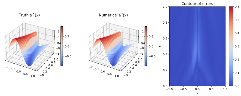
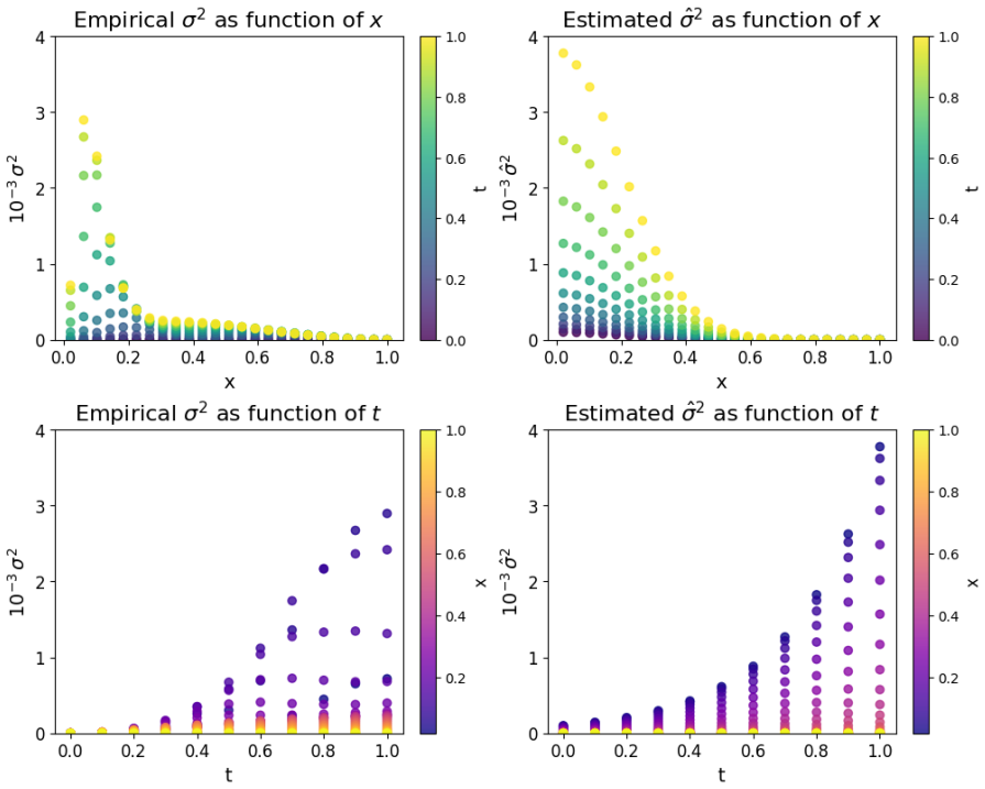
The authors claim that fitting a differentiable non-stationary kernel to an empirical kernel from low-fidelity simulations and then deriving a high-fidelity kernel together with its mean via the multifidelity cokriging framework supplies the necessary ingredients for a Gaussian process to solve nonlinear partial differential equations, with the resulting solver demonstrated on the Burgers' equation.

What carries the argument

The two-step cokriging procedure that fits a non-stationary kernel to a low-fidelity empirical kernel and transfers it to a high-fidelity kernel and mean for use inside a physics-informed Gaussian process.

Load-bearing premise

Empirical kernels extracted from low-fidelity simulations contain transferable information that, when processed through cokriging, produces a high-fidelity kernel and mean suitable for accurate Gaussian process PDE solving.

What would settle it

If the multifidelity method does not produce lower solution error than a single-fidelity Gaussian process on the Burgers' equation under identical high-fidelity data budgets, the central claim would be falsified.

Figures

Figures reproduced from arXiv: 2605.10383 by Fatima-Zahrae El-Boukkouri, Josselin Garnier, Olivier Roustant.

**Figure 2.** Figure 2: MF mean-ker result: L2 error = 0.03 ; max error = 0.13 The numerical solution in [PITH_FULL_IMAGE:figures/full_fig_p013_2.png] view at source ↗

**Figure 3.** Figure 3: MF mean-ker result: L2 error = 0.03 ; max error = 0.13 The reconstructed solution in [PITH_FULL_IMAGE:figures/full_fig_p014_3.png] view at source ↗

**Figure 4.** Figure 4: L2 error = 0.01; max error = 0.09 17 [PITH_FULL_IMAGE:figures/full_fig_p017_4.png] view at source ↗

**Figure 5.** Figure 5: Histogram of errors of the random selection method [PITH_FULL_IMAGE:figures/full_fig_p018_5.png] view at source ↗

**Figure 6.** Figure 6: MF ker-only with non-stationary Gibbs kernel: L2 error = 0.003; max error = 0.02. The result is presented in [PITH_FULL_IMAGE:figures/full_fig_p019_6.png] view at source ↗

**Figure 7.** Figure 7: Solution obtained without interpolation constraints. [PITH_FULL_IMAGE:figures/full_fig_p021_7.png] view at source ↗

**Figure 8.** Figure 8: Solution obtained with interpolation constraints only. [PITH_FULL_IMAGE:figures/full_fig_p021_8.png] view at source ↗

**Figure 9.** Figure 9: Spatially varying α(x) = 1 + 0.2 sin(πx) – MF ker-only (Gibbs kernel): L2 error = 0.02; max error = 0.10. Despite the structural discrepancy between the low- and high-fidelity models, the multifidelity framework remains capable of capturing the main features of the solution. The error levels in [PITH_FULL_IMAGE:figures/full_fig_p023_9.png] view at source ↗

**Figure 10.** Figure 10: Non-stationary Gibbs kernel – MF mean-ker: L2 error = 0.008; max error = 0.03. 26 [PITH_FULL_IMAGE:figures/full_fig_p026_10.png] view at source ↗

**Figure 11.** Figure 11: Non-stationary Gibbs kernel – MF mean-only : L2 error = 0.06; max error = 0.31. Over the 80 independent realizations, the errors obtained with MF mean-ker are L2 = (4.19 ± 0.77) × 10−3 , ∥ · ∥∞ = (3.08 ± 0.95) × 10−2 . For MF mean-only, the corresponding errors are L2 = (5.77 ± 0.0081) × 10−2 , ∥ · ∥∞ = (2.32 ± 0.021) × 10−1 . A.2 Stationary anisotropic Gaussian kernel We now consider the class of station… view at source ↗

**Figure 12.** Figure 12: Stationary Gaussian kernel – MF ker-only (MF ker-only): L2 error = 0.008; max error = 0.04. 27 [PITH_FULL_IMAGE:figures/full_fig_p027_12.png] view at source ↗

**Figure 13.** Figure 13: Stationary Gaussian kernel – MF mean-ker: L2 error = 0.01; max error = 0.08 [PITH_FULL_IMAGE:figures/full_fig_p028_13.png] view at source ↗

**Figure 14.** Figure 14: Stationary Gaussian kernel – MF mean-only: L2 error = 0.05; max error = 0.27. Over the 80 independent realizations, the errors obtained with MF ker-only are L2 = (4.49 ± 0.68) × 10−3 , ∥ · ∥∞ = (3.29 ± 0.71) × 10−2 . For MF mean-ker, the errors are L2 = (4.48 ± 0.68) × 10−3 , ∥ · ∥∞ = (3.26 ± 0.68) × 10−2 . For MF mean-only, the errors are L2 = (5.98 ± 0.0034) × 10−2 , ∥ · ∥∞ = (2.98 ± 0.015) × 10−1 . A.3… view at source ↗

**Figure 15.** Figure 15: Comparison between empirical and estimated variances. [PITH_FULL_IMAGE:figures/full_fig_p029_15.png] view at source ↗

**Figure 16.** Figure 16: Non-stationary Gaussian kernel – MF ker-only: L2 error = 0.008; max error = 0.04 [PITH_FULL_IMAGE:figures/full_fig_p030_16.png] view at source ↗

**Figure 17.** Figure 17: Non-stationary Gaussian kernel – MF mean-ker: L2 error = 0.01; max error = 0.08 [PITH_FULL_IMAGE:figures/full_fig_p030_17.png] view at source ↗

**Figure 18.** Figure 18: Non-stationary Gaussian kernel – MF mean-only: L2 error = 0.02; max error = 0.16. Over the 80 independent realizations, the errors obtained with MF ker-only are L2 = (4.53 ± 0.70) × 10−3 , ∥ · ∥∞ = (3.34 ± 0.75) × 10−2 . 30 [PITH_FULL_IMAGE:figures/full_fig_p030_18.png] view at source ↗

**Figure 19.** Figure 19: Spatially varying α(x) = 1 + 0.2 sin(πx) – MF mean-ker (Gibbs kernel): L2 error = 0.02; max error = 0.11 [PITH_FULL_IMAGE:figures/full_fig_p031_19.png] view at source ↗

**Figure 20.** Figure 20: Spatially varying α(x) = 1 + 0.2 sin(πx) – MF mean-only (Gibbs kernel): L2 error = 0.03; max error = 0.17. As in the previous configurations, MF ker-only remains the most accurate approach, while MF mean-ker and MF mean-only lead to slightly larger errors. This confirms that, even in the presence of a structural discrepancy between low- and high-fidelity models, kernel learning from multifidelity informa… view at source ↗

read the original abstract

Solving nonlinear partial differential equations (PDEs) using kernel methods offers a compelling alternative to traditional numerical solvers. However, the performance of these methods strongly depends on the choice of kernel. In this work, as the available information is inherently multifidelity, we propose a kernel learning approach based on cokriging, leveraging empirical information from multifidelity simulations. In the first step, we fit a differentiable non-stationary kernel to an empirical kernel obtained from low-fidelity simulations. In the second step, we derive a high-fidelity kernel with estimated hyperparameters, and construct a corresponding high-fidelity mean using the multifidelity framework. These components can then be used within a Gaussian process framework for solving PDEs. Finally, we demonstrate the performance of the proposed physics-informed method on the Burgers' equation.

Editorial analysis

A structured set of objections, weighed in public.

Desk editor's note, referee report, simulated authors' rebuttal, and a circularity audit. Tearing a paper down is the easy half of reading it; the pith above is the substance, this is the friction.

Desk Editor's Note private letter to a colleague

This paper gives a workable two-step cokriging recipe to learn a non-stationary kernel and mean from low-fidelity runs for physics-informed GP PDE solvers, and the Burgers example checks out without internal contradictions.

read the letter

The core contribution is a practical pipeline: fit a differentiable non-stationary kernel to the empirical covariance matrix from cheap low-fidelity simulations, then apply cokriging to produce a high-fidelity kernel plus mean that drops straight into a Gaussian-process PDE solver. They test it on Burgers' equation and the numbers line up with the procedure they describe. That is genuinely new as a targeted combination for this setting, and it addresses the real problem that kernel choice often makes or breaks these methods. The approach stays heuristic and empirical, which matches what the work claims rather than over-promising theory. The single numerical check is consistent and shows the low-fidelity information can transfer usefully without obvious breakdown. Soft spots are modest but real. Validation rests on one nonlinear PDE, so we do not yet know how the method behaves on other equations or with different fidelity gaps. Hyperparameters are estimated from the same multifidelity data, which introduces some dependence on fitting choices even if the stress test found no circularity that invalidates the construction. There are no error bounds or extensive baselines against other kernel-learning tricks, which leaves the practical gain somewhat qualitative for now. This paper is for people already building or using kernel-based PDE solvers who need a concrete way to exploit cheap simulations for better kernels. A reader in scientific machine learning would get a recipe worth trying on their own problems. It deserves peer review because the steps are clear, the example supports the claim on its own terms, and the idea targets a genuine bottleneck even if more cases and comparisons would strengthen it.

Referee Report

0 major / 3 minor

Summary. The manuscript proposes a two-step cokriging procedure for learning kernels in a multifidelity Gaussian process framework to solve nonlinear PDEs. Low-fidelity simulations are used to construct an empirical kernel to which a differentiable non-stationary kernel is fit; hyperparameters are then transferred to define a high-fidelity kernel and mean function that are inserted into a physics-informed GP solver. The approach is illustrated on Burgers' equation.

Significance. If the empirical transfer from low- to high-fidelity kernels proves reliable, the method supplies a practical, data-driven route to kernel construction for physics-informed GPs when high-fidelity data are scarce. This could reduce reliance on hand-crafted kernels and improve accuracy for nonlinear PDEs, adding a useful heuristic tool to the scientific machine-learning literature.

minor comments (3)

The abstract summarizes the procedure but omits any equations, error metrics, or quantitative results; adding a brief statement of the observed accuracy on Burgers' equation would improve readability.
Notation for the empirical kernel, the fitted non-stationary kernel, and the derived high-fidelity mean should be introduced once and used consistently; cross-references to the relevant equations would help readers follow the two-step construction.
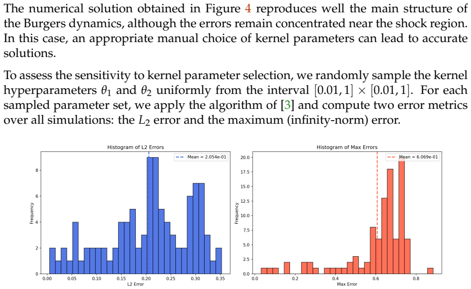
The single numerical example on Burgers' equation is consistent with the stated procedure, but the manuscript would benefit from a short discussion of how sensitive the final GP solution is to the choice of low-fidelity resolution or the number of multifidelity samples.

Simulated Author's Rebuttal

0 responses · 0 unresolved

We thank the referee for their careful summary of our work and for the positive recommendation of minor revision. The report raises no specific major comments or criticisms, so we have nothing to rebut point by point. We will incorporate any minor editorial suggestions in the revised manuscript.

Circularity Check

0 steps flagged

No significant circularity detected in derivation chain

full rationale

The paper describes an empirical two-step cokriging procedure: fitting a differentiable non-stationary kernel to an empirical kernel extracted from low-fidelity simulations, then deriving a high-fidelity kernel and mean via the multifidelity framework for subsequent use in a physics-informed GP PDE solver. This construction is presented as a heuristic that leverages external multifidelity data and standard GP components; it does not reduce any claimed prediction or result to its own fitted inputs by definition, nor does it rely on self-citation load-bearing uniqueness theorems or ansatzes smuggled from prior work. The single numerical demonstration on Burgers' equation is consistent with the stated procedure without internal reduction. The central claim therefore remains independent of its inputs on the paper's own terms.

Axiom & Free-Parameter Ledger

1 free parameters · 2 axioms · 0 invented entities

The approach rests on standard Gaussian process and cokriging assumptions plus the domain claim that low-fidelity empirical kernels transfer usefully to high-fidelity settings; hyperparameters are fitted rather than derived from first principles.

free parameters (1)

high-fidelity kernel hyperparameters
Estimated within the multifidelity cokriging step as described in the abstract.

axioms (2)

domain assumption Gaussian processes with suitable kernels can solve nonlinear PDEs
Invoked when the learned kernel and mean are placed inside the GP framework for PDE solving.
domain assumption Low-fidelity simulation data yields an empirical kernel that is informative for high-fidelity modeling
Core premise of the first step and the subsequent cokriging transfer.

pith-pipeline@v0.9.0 · 5437 in / 1556 out tokens · 42396 ms · 2026-05-12T03:45:13.014149+00:00 · methodology

discussion (0)

Lean theorems connected to this paper

Citations machine-checked in the Pith Canon. Every link opens the source theorem in the public Lean library.

IndisputableMonolith/Cost/FunctionalEquation.lean washburn_uniqueness_aczel unclear
we fit a differentiable non-stationary kernel to an empirical kernel obtained from low-fidelity simulations... k∗H=ρ²kopt+kd
IndisputableMonolith/Foundation/AlexanderDuality.lean alexander_duality_circle_linking unclear
non-stationary Gibbs kernel... Σx=diag(ℓ1(x),ℓ2(x))

Reference graph

Works this paper leans on

30 extracted references · 30 canonical work pages

[1]

Argyriou, C

A. Argyriou, C. A. Micchelli, and M. Pontil. When is there a representer theo- rem? Vector versus matrix regularizers.The Journal of Machine Learning Research, 10:2507–2529, 2009

work page 2009
[2]

S. C. Brenner and L. R. Scott.The mathematical theory of finite element methods. Springer, 2008

work page 2008
[3]

Y. Chen, B. Hosseini, H. Owhadi, and A. M. Stuart. Solving and learning nonlin- ear PDEs with Gaussian processes.Journal of Computational Physics, 447:110668, 2021

work page 2021
[4]

Cockayne, C

J. Cockayne, C. Oates, T. Sullivan, and M. Girolami. Bayesian probabilistic nu- merical methods.SIAM Review, 61(4):756–789, 2019

work page 2019
[5]

Cressie.Statistics for spatial data

N. Cressie.Statistics for spatial data. Wiley, 1993

work page 1993
[6]

Doumèche, F

N. Doumèche, F. Bach, G. Biau, and C. Boyer. Physics-informed kernel learning. Journal of Machine Learning Research, 26(124):1–39, 2025

work page 2025
[7]

El-Boukkouri, J

F.-Z. El-Boukkouri, J. Garnier, and O. Roustant. General reproducing properties in RKHS with application to derivative and integral operators.arXiv preprint arXiv:2503.15922, 2025

work page arXiv 2025
[8]

L. C. Evans.Partial differential equations, volume 19. American mathematical soci- ety, 2022

work page 2022
[9]

G. E. Fasshauer.Meshfree approximation methods with Matlab (With Cd-rom), vol- ume 6. World Scientific Publishing Company, 2007. 24

work page 2007
[10]

A. I. J. Forrester, A. Sóbester, and A. J. Keane. Multi-fidelity optimization via surrogate modelling.Proceedings of the Royal Society A, 463(2088):3251–3269, 2007

work page 2088
[11]

M. N. Gibbs.Bayesian Gaussian processes for regression and classification. PhD thesis, University of Cambridge, UK, 1998

work page 1998
[12]

Grossmann, H.-G

C. Grossmann, H.-G. Roos, and M. Stynes.Numerical Treatment of Partial Differen- tial Equations: translated and revised by Martin Stynes. Springer, 2007

work page 2007
[13]

E. Hopf. The partial differential equationu t +uu x =µu xx.Communications on Pure and Applied Mathematics, 3(3):201–230, 1950

work page 1950
[14]

G. E. Karniadakis, I. G. Kevrekidis, L. Lu, P . Perdikaris, S. Wang, and L. Yang. Physics-informed machine learning.Nature Reviews Physics, 3(6):422–440, 2021

work page 2021
[15]

M. C. Kennedy and A. O’Hagan. Predicting the output from a complex computer code when fast approximations are available.Biometrika, 87(1):1–13, 2000

work page 2000
[16]

Le Gratiet.Multi-fidelity Gaussian process regression for computer experiments

L. Le Gratiet.Multi-fidelity Gaussian process regression for computer experiments. PhD thesis, Université Paris-Diderot, 2013

work page 2013
[17]

N. H. Nelsen, H. Owhadi, A. M. Stuart, X. Yang, and Z. Zou. Bilevel optimization for learning hyperparameters: Application to solving PDEs and inverse problems with Gaussian processes.arXiv preprint arXiv:2510.05568, 2025

work page arXiv 2025
[18]

C. J. Paciorek and M. J. Schervish. Spatial modelling using a new class of nonsta- tionary covariance functions.Environmetrics: The official journal of the International Environmetrics Society, 17(5):483–506, 2006

work page 2006
[19]

Peherstorfer, K

B. Peherstorfer, K. Willcox, and M. Gunzburger. Survey of multifidelity methods in uncertainty propagation, inference, and optimization.SIAM Review, 60(3):550– 591, 2018

work page 2018
[20]

Pigoli, J

D. Pigoli, J. A. Aston, I. L. Dryden, and P . Secchi. Distances and inference for covariance operators.Biometrika, 101(2):409–422, 2014

work page 2014
[21]

Quarteroni and A

A. Quarteroni and A. Valli.Numerical approximation of partial differential equations. Springer, 1994

work page 1994
[22]

Raissi, P

M. Raissi, P . Perdikaris, and G. E. Karniadakis. Physics-informed neural net- works: A deep learning framework for solving forward and inverse problems in- volving nonlinear partial differential equations.Journal of Computational physics, 378:686–707, 2019

work page 2019
[23]

Seydao˘ glu, U

M. Seydao˘ glu, U. Erdo˘ gan, and T. Özi¸ s. Numerical solution of Burgers’ equation with high order splitting methods.Journal of Computational and Applied Mathemat- ics, 291:410–421, 2016

work page 2016
[24]

M. L. Stein.Interpolation of spatial data. Springer, 1999

work page 1999
[25]

A. M. Stuart. Inverse problems: A Bayesian perspective.Acta Numerica, 19:451– 559, 2010

work page 2010
[26]

Z. Wang, W. Xing, R. Kirby, and S. Zhe. Physics informed deep kernel learning. InInternational conference on artificial intelligence and statistics, pages 1206–1218. PMLR, 2022. 25

work page 2022
[27]

Wendland.Scattered Data Approximation

H. Wendland.Scattered Data Approximation. Cambridge University Press, 2004

work page 2004
[28]

Williams and C

C. Williams and C. Rasmussen. Gaussian Processes for Machine Learning, MIT Press.Cambridge, MA, 2006

work page 2006
[29]

X. Yang, G. Tartakovsky, and A. Tartakovsky. Physics-information-aided krig- ing: Constructing covariance functions using stochastic simulation models.arXiv preprint arXiv:1809.03461, 2018

work page arXiv 2018
[30]

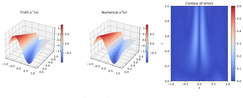
X. Yang, X. Zhu, and J. Li. When bifidelity meets cokriging: An efficient physics- informed multifidelity method.SIAM Journal on Scientific Computing, 42(1):A220– A249, 2020. A Additional numerical results for the Burgers’ equa- tion In this appendix, we report additional numerical results obtained for the Burgers’ equation in the multifidelity setting. A...

work page 2020