arxiv: 2605.10552 · v1 · submitted 2026-05-11 · 🧮 math.DS

Recognition: 3 theorem links

· Lean Theorem

Hausdorff Dimension of a Class of Self-Affine Sets

Amal P. S., Ramkumar P. B, Vinod Kumar P. B.

Pith reviewed 2026-05-12 03:44 UTC · model grok-4.3

classification 🧮 math.DS

keywords self-affine setsHausdorff dimensioniterated function systemsopen set conditionaffine mapssimilaritiesattractors

0 comments

The pith

Self-affine attractors with eventually similar maps and commuting linear parts have exact Hausdorff dimensions under the open set condition.

A machine-rendered reading of the paper's core claim, the machinery that carries it, and where it could break.

The paper derives exact Hausdorff dimension formulas for attractors of iterated function systems that include an affine map whose iterates eventually become similarities, together with similarities whose linear parts commute with the symmetric operator A transpose A. This class is extended to hybrid systems with multiple such maps and to cases with exact overlaps. A reader would care because these conditions allow precise dimension calculations for self-affine sets, which are otherwise difficult to determine exactly. The work also classifies the topology in the plane, showing that for two maps the relation between their contraction ratios c and r must satisfy c plus r equals one to guarantee both the open set condition and connectedness of the attractor.

Core claim

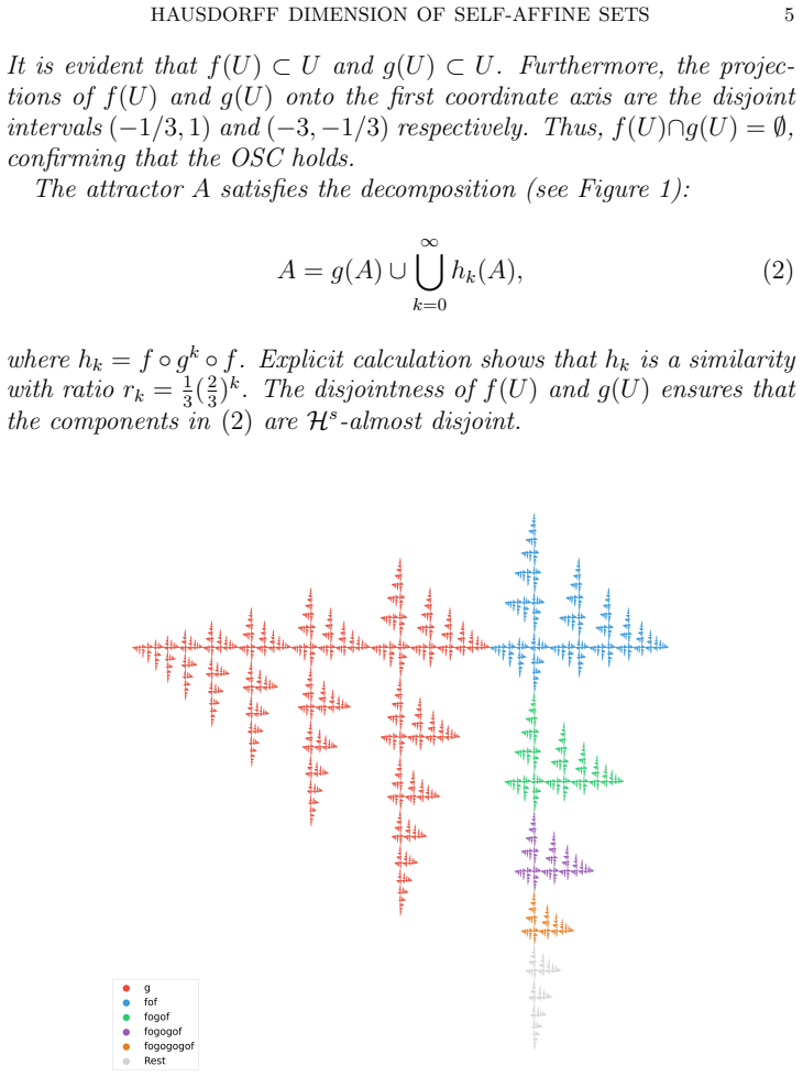
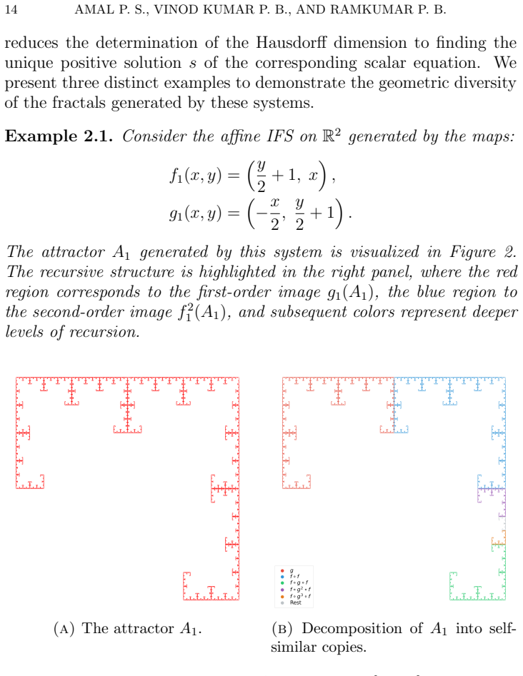
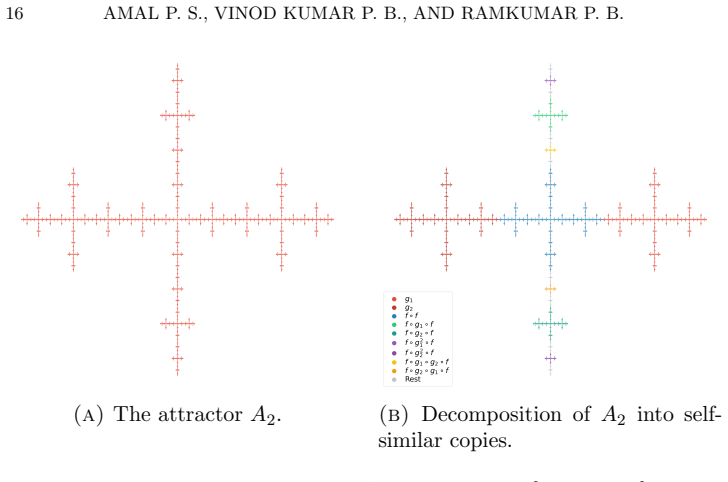
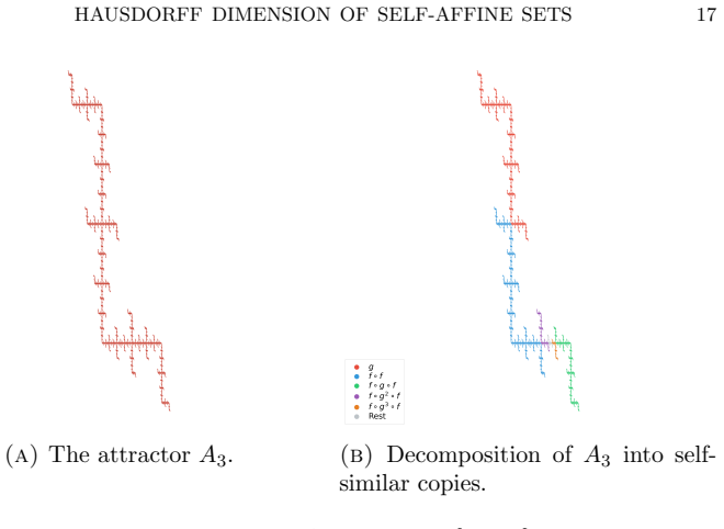
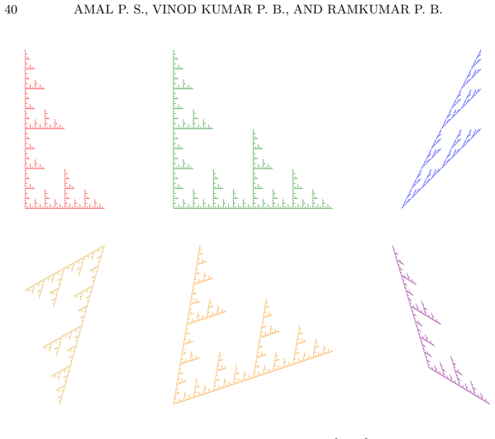
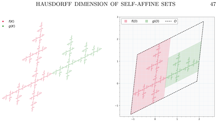
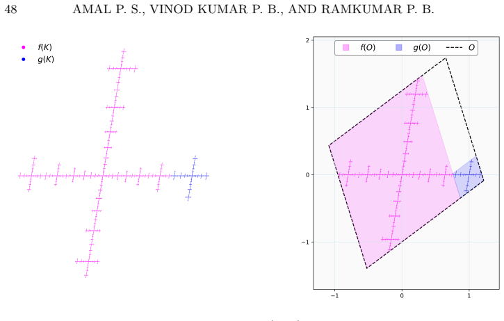
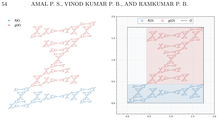
For a class of self-affine attractors generated by affine iterated function systems containing an affine map whose n-th iterate is a similarity contraction and standard similarities whose linear parts commute with the symmetric operator A transpose A, the attractor exists uniquely and under the open set condition its exact Hausdorff dimension is computed. The framework extends to systems where all map compositions of some fixed length are similarities, to systems with overlaps that are exact homothetic copies, and to hybrid systems combining multiple eventually contractive affine maps with universally aligned similarities. In the plane, for a two-map system with contraction ratios c and r, c

What carries the argument

The commuting condition of the linear parts of the similarities with the symmetric operator A transpose A derived from the affine map, which enables the exact dimension calculation by allowing the system to behave like a similarity system in key respects.

If this is right

The attractor exists and is unique for the systems considered.
Exact Hausdorff dimension is obtained under the open set condition.
The results unify to give dimension formulas for hybrid systems with multiple affine maps and aligned similarities.
For two-map systems in the plane the parameter balance c plus r equals one uniquely ensures the open set condition and connectedness.

Where Pith is reading between the lines

These are editorial extensions of the paper, not claims the author makes directly.

The commuting requirement implies that the maps must be specially aligned, so the formulas apply only to non-generic choices of linear parts.
The topological bottleneck identified in the plane suggests that similar parameter relations could be sought in higher dimensions to control connectedness.
These special cases may serve as test beds for verifying numerical methods for computing dimensions of more general self-affine sets.

Load-bearing premise

The linear parts of the standard similarities commute with the symmetric operator A transpose A, where A is the linear part of the affine map.

What would settle it

An explicit two-map system with contraction ratios c and r where c plus r does not equal one, yet the open set condition still holds or the attractor is connected, would falsify the claim that this balance is the unique guarantor.

Figures

Figures reproduced from arXiv: 2605.10552 by Amal P. S., Ramkumar P. B, Vinod Kumar P. B..

**Figure 1.** Figure 1: The attractor A decomposed into self-similar subsets. The large red region is the image g(A). The remaining sequence of smaller regions corresponds to the images under the maps f ◦ g k ◦ f for k ≥ 0. Let s = dimH(A). Applying the s-dimensional Hausdorff measure Hs to (2) and using the scaling property Hs (T(E)) = c sHs (E) for [PITH_FULL_IMAGE:figures/full_fig_p005_1.png] view at source ↗

**Figure 2.** Figure 2: The attractor A1 of the IFS {f1, g1} from Example 2.1. The multicolor plot (b) highlights the recursive structure: Red is g1(A1), Blue is f 2 1 (A1), etc. We verify that the system satisfies the conditions of Theorem 1.4: (1) The map f1 has the linear part Mf1 = 0 0.5 1 0 . Although f1 permutes and scales coordinates differently, its second iterate f 2 1 acts as a similarity with ratio c = 1/2. Thus, … view at source ↗

**Figure 3.** Figure 3: The attractor A2 of the IFS {f2, g2a, g2b} from Example 2.2. The right panel (b) visualizes the recursive decomposition into self-similar copies, where the colored regions represent the constituent components generated by the system. Example 2.3. We consider a third system defined by the maps: f3(x, y) = y 4 , 2x , g3(x, y) = − x 2 , − y 2 + 1 . The attractor A3 is displayed in [PITH_FULL_IMAGE:figu… view at source ↗

**Figure 4.** Figure 4: The attractor A3 of the IFS {f3, g3} from Example 2.3. The right panel (b) identifies the components g3(A3) and f 2 3 (A3), along with various smaller self-similar copies that constitute the attractor. This equation is identical to the one derived in Example 2.1. Consequently, the Hausdorff dimension is the same: s = 2 log2 (φ) ≈ 1.388. Example 2.4. Consider the affine IFS on R 2 generated by the maps: f… view at source ↗

**Figure 5.** Figure 5: The attractor A4 of the IFS {f4, g4a, g4b} from Example 2.4. The colors correspond to the disjoint images of the attractor under the generating maps: f4(A4) is shown in blue, g4a(A4) in red, and g4b(A4) in green. Solving numerically yields s ≈ 1.713. 3. Example: Importance of the Alignment Condition The f-aligned condition in Theorem 1.4 is not merely a simplifying assumption but an essential geometric co… view at source ↗

**Figure 6.** Figure 6: The attractor of the IFS {f, g, h}. The structure contains a subset whose vertical projection is the interval [−4, 4], demonstrating that dimH(A) ≥ 1. 3.1. Verification of Parameters and OSC [PITH_FULL_IMAGE:figures/full_fig_p019_6.png] view at source ↗

**Figure 7.** Figure 7: The attractor of the system {f, g}. The coloring distinguishes the four second-level images (f 2 , fg, gf, g2 ), demonstrating the separation of components required by the Open Set Condition. Example 4.2. Consider the system defined by the four affine maps on R 2 : f1(x, y) = (y/4 − 1, −x), g1(x, y) = (−y/4 + 1, x), h1(x, y) = (−y/4, x + 2), k1(x, y) = (y/4, −x + 2). The linear parts of these maps are ort… view at source ↗

**Figure 8.** Figure 8: The attractor of the overlapping system {f1, g1, h1, k1}. The Open Set Condition fails as h1(A) and k1(A) intersect. The plot decomposes the set into components: Blue (f1(A)), Green (g1(A)), Red (h1(A) \ k1(A)), Orange (k1(A) \ h1(A)), and the overlap region in Purple (h1(A) ∩ k1(A)). intersection h2(A) ∩ k2(A) forms a self-similar copy of the attractor scaled by the factor p = 1/5. Since f2(A) and g2(A) a… view at source ↗

**Figure 9.** Figure 9: The attractor of the system {f2, g2, h2, k2}. The images f2(A) (Blue) and g2(A) (Green) are strictly disjoint from the rest of the set. The only overlap occurs between h2(A) (Red) and k2(A) (Orange) near the origin. The intersection region h2(A) ∩ k2(A) is highlighted in purple. Substituting the values: 4 1 5 s/2 − 1 5 s = 1. Let x = (1/5)s/2 . The equation becomes: 4x − x 2 = 1 =⇒ x 2 − 4x + 1 = 0. … view at source ↗

**Figure 10.** Figure 10: The attractor of the hybrid system defined in Example 5.1. The red region corresponds to the map f1, the blue region corresponds to the map f2, and the green region corresponds to the map g1. The affine maps are defined by: f1(x, y) = −y, x 2 , f2(x, y) = y 2 , x 4 + 1 , f3(x, y) = − y 2 , − x 4 − 1 . The similarity maps are defined by: g1(x, y) = x 4 + 1, y 4 + 1 , g2(x, y) = x 4 − 1, y 4 − … view at source ↗

**Figure 11.** Figure 11: The attractor of the hybrid system defined in Example 5.2. The red structure corresponds to f1, blue to f2, green to f3, while gold and violet correspond to the similarities g1 and g2. The four compositions f 2 2 , f 2 3 , f2 ◦ f3, and f3 ◦ f2 are similarities with ratio 1/8. The maps g1 and g2 are standard similarities with ratio r1 = r2 = 1/4. The system satisfies the Open Set Condition with the open se… view at source ↗

**Figure 12.** Figure 12: Attractors of the IFS {f, g} for various translation vectors: (Red) bf = (0, 0), bg = (0, 0.5); (Green) bf = (0, 0.5), bg = (1, 0.5); (Blue) bf = (−0.5, 0), bg = (0, 0.5); (Gold) bf = (0.2, −0.2), bg = (−0.8, −3.2); (Orange) bf = (0, 0), bg = (3, 1); (Purple) bf = (0, 0.5), bg = (0.1, 1). As shown in [PITH_FULL_IMAGE:figures/full_fig_p040_12.png] view at source ↗

**Figure 13.** Figure 13: Geometric validation of the Open Set Condition for Example 6.1 (A2 = −cI, S = rI). The left panel displays the attractor K = f(K) ∪ g(K). The right panel illustrates the rigorously constructed Euclidean bounding set O, mapped from the theoretical dual axes, alongside its strictly disjoint affine images f(O) and g(O). This provides direct geometric corroboration of the algebraic separation guarantees, c… view at source ↗

**Figure 14.** Figure 14: The attractor (left) and the Euclidean bounding set O (right) for Example 6.2. The lack of interior overlap between the regions f(O) and g(O) provides visual proof of the open set condition. (3) c + r ≤ 1. (4) The respective fixed points zf and zg of f and g are distinct, and the attractor K is not contained in a single 1-dimensional line. Then F satisfies the open set condition. Proof. Let zf , zg ∈ R 2… view at source ↗

**Figure 15.** Figure 15: The attractor (left) and bounding set O (right) for Example 6.3. The lack of interior overlap between f(O) and g(O) provides direct geometric proof of the open set condition. Mapping these boundaries back to R 2 via the inverse projection matrix P −1 yields the vertices for the bounding set O: v1 = 1.75 1.75 , v2 = 1.75 0 , v3 = 0 0 , v4 = 0 1.75 . Thus, the bounding set O corresponds to a… view at source ↗

**Figure 16.** Figure 16: The attractor (left) and the bounding square O (right) for Example 6.4. The images f(O) and g(O) demonstrate strict interior separation without overlap, geometrically validating the open set condition. (2) If c + r < 1, then K is totally disconnected. Proof. Let zf , zg ∈ R 2 denote the distinct fixed points of f and g. The infinite line passing through zf and zg is invariant under the subsystem {f 2 , g… view at source ↗

**Figure 17.** Figure 17: Failure of the Open Set Condition when S is an axial reflection. In both examples, the parameters satisfy c = 1/5, r = 4/5, and the constraint c + r ≤ 1, yet the sets f(K) and g(K) overlap. The sum of the parameters is c + r = 7/6 > 1. If S were a uniform scaling or point reflection, Theorem 6.5 would guarantee a connected attractor. However, the attractor here is totally disconnected (see Figure 18), co… view at source ↗

**Figure 18.** Figure 18: The attractor of the IFS defined in Example 6.7, illustrating the failure of connectedness under axial reflection. Although the parameters c = 2/3 and r = 1/2 satisfy c + r > 1, the orientation-reversing nature of S results in a totally disconnected set. Junior Research Fellowship (JRF) (Ref. No. [1090(CSIR-UGC NET JUNE 2019)]) awarded to the first author. The first and third authors acknowledge the insti… view at source ↗

read the original abstract

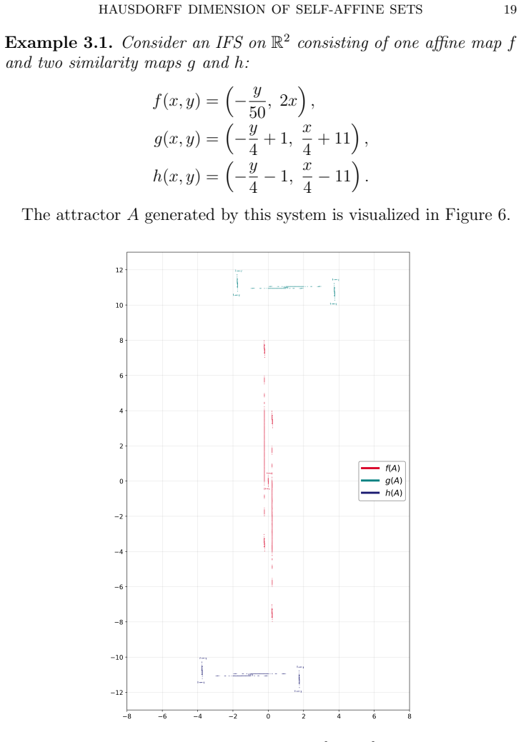
In this paper, exact Hausdorff dimension formulas for a class of self-affine attractors generated by affine Iterated Function Systems are derived. We consider systems containing an affine map whose $n$-th iterate is a similarity contraction, alongside standard similarities whose linear parts commute with the symmetric operator $A^\top A$, where $A$ is the linear part of the affine map. We prove that the attractor of such a system exists uniquely, and, under the Open Set Condition, we compute its exact Hausdorff dimension. We extend this framework to systems where all map compositions of some fixed length are similarities, and to systems where overlaps are exact homothetic copies of the attractor. We unify these approaches to establish dimension formulas for hybrid systems that combine multiple eventually contractive affine maps with universally aligned similarities. Finally, we conclude with a topological classification of these systems in the plane. For a two-map system comprising an affine map whose second iterate is a similarity with contraction ratio $c$, alongside an $f$-aligned similarity with ratio $r$, we prove that the precise parameter balance $c + r = 1$ acts as a strict topological bottleneck uniquely guaranteeing both the open set condition and the connectedness of the attractor.

Editorial analysis

A structured set of objections, weighed in public.

Desk editor's note, referee report, simulated authors' rebuttal, and a circularity audit. Tearing a paper down is the easy half of reading it; the pith above is the substance, this is the friction.

Desk Editor's Note private letter to a colleague

The paper gives exact Hausdorff dimension formulas for a restricted hybrid class of self-affine IFS that mix eventually contractive affine maps with commuting similarities.

read the letter

The punchline is that this work delivers explicit Hausdorff dimension formulas for self-affine sets from a new but narrowly defined class of iterated function systems. The systems mix one affine map that turns into a similarity after a fixed number of iterations with standard similarities whose linear parts commute with the symmetric operator coming from the affine map's linear part. They also establish that in the two-map planar setting, the relation c + r = 1 is the precise condition that guarantees both the open set condition and connectedness of the attractor. The paper does well by bringing together eventually contractive affine maps, commuting similarities, and exact overlap cases into a single framework. This unification allows them to handle hybrid systems and derive the dimension from the singular value pressure under the open set condition. The topological classification for the two-map case is a clean result that pins down when the attractor behaves nicely. The stress-test confirms that the central claims hold without internal inconsistencies once the commuting condition is accepted as part of the definition. The soft spots are mostly about scope. The commuting condition with A transpose A is restrictive and will not hold for most choices of maps, so the exact formulas apply only inside this subclass. The topological bottleneck is proved only for two maps in the plane, which limits how far the classification extends. These are not hidden flaws but explicit boundaries on the results. No problems with circular reasoning or unverified steps appear in the derivations. This paper is aimed at researchers in fractal geometry and dynamical systems who focus on computing dimensions for self-affine attractors. A reader familiar with the open set condition and pressure functions will appreciate the concrete formulas and the way the authors extend prior techniques. It is not revolutionary, but it fills in a gap for these hybrid systems. I would bring it to a reading group to go over the commuting assumption and the proof of the c + r = 1 condition. The work shows honest engagement with the literature and clear thinking on its own terms. It deserves a serious referee because the results are grounded and the evidence supports the claims within the restricted class.

Referee Report

0 major / 3 minor

Summary. The paper derives exact Hausdorff dimension formulas for self-affine attractors generated by affine IFSs that include an affine map whose n-th iterate is a similarity contraction together with standard similarities whose linear parts commute with the symmetric operator A^T A (A the linear part of the affine map). It establishes existence and uniqueness of the attractor, computes the precise dimension under the open set condition (OSC), extends the framework to systems in which all compositions of fixed length are similarities and to cases of exact homothetic overlaps, unifies these for hybrid systems combining multiple eventually contractive affine maps with aligned similarities, and concludes with a planar topological classification: for a two-map system with an affine map whose second iterate is a similarity of ratio c and an f-aligned similarity of ratio r, the relation c + r = 1 is the unique parameter balance that simultaneously guarantees the OSC and connectedness of the attractor.

Significance. If the results hold, the work supplies rare closed-form dimension expressions for a nontrivial subclass of self-affine sets by exploiting the commuting condition to reduce the singular-value pressure to an explicitly solvable equation under OSC. The unification across eventually-similar, exact-overlap, and hybrid cases, together with the explicit identification of c + r = 1 as a strict topological bottleneck linking dimension theory to connectedness, constitutes a concrete advance within the restricted class of systems defined by the commuting and eventual-similarity hypotheses.

minor comments (3)

The abstract introduces the term “f-aligned similarity” without a preliminary definition; a one-sentence clarification of this alignment condition (presumably with respect to the fixed point or the linear part A) should appear in the introduction or the statement of the main theorems.
In the extension to hybrid systems, the manuscript should explicitly record whether the OSC assumed for the individual subsystems is inherited by the combined IFS or whether a separate verification is required; a short paragraph or remark after the unification theorem would remove any ambiguity.
The topological classification is stated for planar two-map systems; a brief remark on whether the c + r = 1 bottleneck extends verbatim to higher-dimensional analogues (or why it does not) would help readers assess the scope of the result.

Simulated Author's Rebuttal

0 responses · 0 unresolved

We thank the referee for the careful summary of our results on exact Hausdorff dimensions for self-affine attractors under the stated hypotheses (eventual similarities, commuting linear parts, OSC), as well as for the positive assessment of the unification across eventually-similar, exact-overlap, and hybrid cases and the planar topological classification. We appreciate the recognition that the commuting condition permits an explicit solution of the singular-value pressure equation.

Circularity Check

0 steps flagged

No significant circularity identified

full rationale

The derivation proceeds by defining a restricted class of IFS (affine maps whose iterates are similarities, plus similarities whose linear parts commute with A^T A) and then applying standard singular-value pressure techniques under the explicitly assumed OSC to obtain explicit dimension formulas. The two-map topological result (c + r = 1 as the unique balance forcing both OSC and connectedness) is proved directly from the planar geometry and second-iterate similarity assumption without reducing to prior self-citations or fitted parameters. All load-bearing steps remain within the stated hypotheses and do not equate the output dimension to an input by construction or rename a known empirical pattern.

Axiom & Free-Parameter Ledger

0 free parameters · 2 axioms · 0 invented entities

The central claims rest on the open set condition as a domain assumption and standard properties of Hausdorff measure and iterated function systems; no free parameters or invented entities are introduced.

axioms (2)

domain assumption Open Set Condition holds for the IFS
Invoked to obtain the exact Hausdorff dimension formula and to guarantee the topological properties.
domain assumption Linear parts of similarities commute with A^T A
Required for the dimension calculation in the main class of systems.

pith-pipeline@v0.9.0 · 5521 in / 1341 out tokens · 28723 ms · 2026-05-12T03:44:51.329230+00:00 · methodology

discussion (0)

Lean theorems connected to this paper

Citations machine-checked in the Pith Canon. Every link opens the source theorem in the public Lean library.

IndisputableMonolith/Constants/AlphaDerivationExplicit.lean phi_golden_ratio echoes
Substituting u = (1/2)^{s/2} yields the quadratic equation u² + u − 1 = 0. The positive solution is the inverse of the Golden Ratio, u = 1/φ = (√5 − 1)/2. Solving for s, we find the exact dimension s = 2 log₂(φ) ≈ 1.388.
IndisputableMonolith/Cost/FunctionalEquation.lean washburn_uniqueness_aczel echoes
c^{s/n} + ∑ r_i^s = 1 (under f-alignment and OSC)
IndisputableMonolith/Foundation/BranchSelection.lean branch_selection refines
the precise parameter balance c + r = 1 acts as a strict topological bottleneck uniquely guaranteeing both the open set condition and the connectedness of the attractor

Reference graph

Works this paper leans on

18 extracted references · 18 canonical work pages

[1]

P. S. Amal, P. B. Vinod Kumar, and P. B. Ramkumar,G-contractions and g-iterated function system, Chaos, Solitons & Fractals209(2026), 118406

work page 2026
[2]

3, 601–659

Bal´ azs B´ ar´ any, Michael Hochman, and Ariel Rapaport,Hausdorff dimension of planar self-affine sets and measures, Inventiones mathematicae216(2019), no. 3, 601–659

work page 2019
[3]

1, 223–244

Bal´ azs B´ ar´ any, Antti K¨ aenm¨ aki, and Henna Koivusalo,Dimension of self-affine sets for fixed translation vectors, Journal of the London Mathematical Society 98(2018), no. 1, 223–244

work page 2018
[4]

10, 4427–4440

Bal´ azs B´ ar´ any, Micha l Rams, and K´ aroly Simon,On the dimension of self-affine sets and measures with overlaps, Proceedings of the American Mathematical Society144(2016), no. 10, 4427–4440

work page 2016
[5]

HAUSDORFF DIMENSION OF SELF-AFFINE SETS 59

Michael F Barnsley,Fractals everywhere, new edition ed., Academic Press, 2014. HAUSDORFF DIMENSION OF SELF-AFFINE SETS 59

work page 2014
[6]

Michael F Barnsley and Stephen Demko,Iterated function systems and the global construction of fractals, Proceedings of the Royal Society of London. A. Mathematical and Physical Sciences399(1985), no. 1817, 243–275

work page 1985
[7]

7, 1975–1977

Michael F Barnsley, V Ervin, D Hardin, and J Lancaster,Solution of an inverse problem for fractals and other sets, Proceedings of the National Academy of Sciences83(1986), no. 7, 1975–1977

work page 1986
[8]

Kenneth Falconer,Fractal geometry: Mathematical foundations and applica- tions, 3rd ed., John Wiley & Sons, Chichester, UK, 2014

work page 2014
[9]

4, 1369–1388

Kenneth Falconer and Tom Kempton,Planar self-affine sets with equal haus- dorff, box and affinity dimensions, Ergodic Theory and Dynamical Systems38 (2018), no. 4, 1369–1388

work page 2018
[10]

2, 339–350

Kenneth J Falconer,The hausdorff dimension of self-affine fractals, Mathe- matical Proceedings of the Cambridge Philosophical Society103(1988), no. 2, 339–350

work page 1988
[11]

7, 2361–2441

Michael Hochman and Ariel Rapaport,Hausdorff dimension of planar self- affine sets and measures with overlaps, Journal of the European Mathematical Society24(2022), no. 7, 2361–2441

work page 2022
[12]

1, 77–97

Irene Hueter and Steven P Lalley,Falconer’s formula for the hausdorff dimen- sion of a self-affine set inR 2, Ergodic Theory and Dynamical Systems15 (1995), no. 1, 77–97

work page 1995
[13]

5, 713–747

John E Hutchinson,Fractals and self-similarity, Indiana University Mathemat- ics Journal30(1981), no. 5, 713–747

work page 1981
[14]

2, 519–544

Thomas Jordan, Mark Pollicott, and K´ aroly Simon,Hausdorff dimension for randomly perturbed self affine attractors, Communications in Mathematical Physics270(2007), no. 2, 519–544

work page 2007
[15]

1, 15–23

Patrick AP Moran,Additive functions of intervals and hausdorff measure, Mathematical Proceedings of the Cambridge Philosophical Society42(1946), no. 1, 15–23

work page 1946
[16]

3, 1547–1582

Ian D Morris and Pablo Shmerkin,On equality of hausdorff and affinity di- mensions, via self-affine measures on positive subsystems, Transactions of the American Mathematical Society371(2019), no. 3, 1547–1582

work page 2019
[17]

2, 1029–1066

Roger D Nussbaum, Amit Priyadarshi, and Sjoerd Verduyn Lunel,Positive op- erators and hausdorff dimension of invariant sets, Transactions of the American Mathematical Society364(2012), no. 2, 1029–1066

work page 2012
[18]

1, 111–115

Andreas Schief,Separation properties for self-similar sets, Proceedings of the American Mathematical Society122(1994), no. 1, 111–115. 60 AMAL P. S., VINOD KUMAR P. B., AND RAMKUMAR P. B. APJ Abdul Kalam Technological University, Thiruvananthapuram, Kerala, India; Rajagiri School of Engineering and Technology, Kochi, Kerala, India Email address:amalb9111@...

work page 1994