arxiv: 2605.10620 · v1 · submitted 2026-05-11 · 🌀 gr-qc · hep-th· math-ph· math.MP

Recognition: no theorem link

The Dirac field in LRS space-times: a covariant approach

Stefano Vignolo , Giuseppe De Maria , Sante Carloni , Luca Fabbri

Authors on Pith no claims yet

Pith reviewed 2026-05-12 04:38 UTC · model grok-4.3

classification 🌀 gr-qc hep-thmath-phmath.MP

keywords Dirac fieldLRS space-timescovariant formalism1+1+2 decompositionpolar decompositionspinorial fluidself-gravitating fields

0 comments

The pith

The Dirac field can be consistently embedded as a self-gravitating source in LRS space-times of types I, II and III using a covariant (1+1+2) formalism.

A machine-rendered reading of the paper's core claim, the machinery that carries it, and where it could break.

The paper develops a description of the Dirac field as an effective spinorial fluid via its polar decomposition. It builds a (1+1+2) covariant formalism that encodes the field equations without tetrads or Clifford matrices. The work then derives the symmetry conditions required for this field to source gravity consistently in locally rotationally symmetric spacetimes. Explicit analytical and numerical solutions are constructed to show the framework in action. A reader would care because the method offers a direct way to include spinor matter in symmetric cosmological models.

Core claim

By extending prior work and requiring that the Dirac velocity and spin vectors lie in the planes of the time-like and space-like congruences, a (1+1+2) covariant formalism is constructed for the self-gravitating Dirac field. This allows consistent embedding in LRS space-times of types I, II and III while satisfying the coupled Einstein-Dirac system, and yields both analytical and numerical solutions.

What carries the argument

The (1+1+2) covariant formalism for the Dirac field based on its polar decomposition as a spinorial fluid, which encodes LRS symmetry directly in the congruence planes.

If this is right

A self-gravitating Dirac field satisfies the symmetry requirements of LRS space-times of types I, II and III under the stated alignment.
Analytical solutions exist for the coupled system in these backgrounds.
Numerical solutions can be generated to explore the dynamics of the spinorial fluid.
The formalism permits direct computation of the energy-momentum tensor from the fluid variables without auxiliary frames.

Where Pith is reading between the lines

These are editorial extensions of the paper, not claims the author makes directly.

The same decomposition could be tested in other symmetry classes such as Bianchi models or spherically symmetric spacetimes.
Stability analysis of the numerical solutions against small perturbations could reveal viable cosmological histories.
Coupling the formalism to additional matter fields might produce new classes of exact solutions for mixed fermionic and bosonic sources.

Load-bearing premise

The velocity and spin vector fields of the Dirac field lie in the planes defined pointwise by the generators of the time-like and space-like congruences.

What would settle it

An explicit LRS metric of type I, II or III together with a Dirac field solution that satisfies the Einstein-Dirac equations while having velocity or spin vectors outside the allowed congruence planes would show the alignment assumption is unnecessary.

Figures

Figures reproduced from arXiv: 2605.10620 by Giuseppe De Maria, Luca Fabbri, Sante Carloni, Stefano Vignolo.

**Figure 1.** Figure 1: Time evolution of the solution (133) with initial data: m = 1, Θ(0) = 1, ρ(0) = 1, η(0) = 1 and β(0) = 0. On the left-hand side: corresponding behavior of the energy density µ (dotted line), the modulus ρ (dashed line) and the expansion scalar Θ (solid line). On the right-hand side: evolution of η (solide line) and β (dashed line). The figure shows that the functions ρ, η and β are indeed oscillating while… view at source ↗

**Figure 2.** Figure 2: Evolution of the system (134) starting from the initial data m = 1, A0 = 0, Ω0 = −1, ϕ0 = ρ0 = η0 = 1 and β0 = π. Left-hand panel: behavior of the kinematical variables A (solid line), ϕ (dotted line), and Ω (dashed line) in function of x. Right-hand panel: behavior of the energy density µ (solid line), radial pressure pr (dashed line), and orthogonal pressure po (dotted line) as functions of x. The plots … view at source ↗

**Figure 3.** Figure 3: Evolution of the system (134) with initial data m = 1, A0 = 0, Ω0 = −1, ϕ0 = ρ0 = η0 = 1 and β0 = π. Left-hand panel: dynamical behavior of the modulus ρ (solid line), the pseudo-scalar function η (dashed line) and the chiral angle β (dotted line) in function of x. Right-hand panel: behavior of the bilinear scalar ψψ¯ (solid line) and the pseudo-scalar iψγ¯ 5ψ (dashed line) as functions of x. The numerical… view at source ↗

**Figure 4.** Figure 4: Dynamical evolution of the system (135) with m = 1 and initial data Θ(t = 1.6) = ρ(t = 1.6) = η(t = 1.6) = 1, Σ(t = 1.6) = 10−5 , β(t = 1.6) = 0. Left-hand panel: behavior of the kinematical variables Θ (solid line), Σ (dotted line) in function of the affine parameter t. Right-hand panel: behavior of the energy density µ (solid line) and the electric part E (dashed line) of the Weyl tensor as functions of … view at source ↗

**Figure 5.** Figure 5: Dynamical evolution of the system (135) with m = 1 and initial data Θ(t = 1.6) = ρ(t = 1.6) = η(t = 1.6) = 1, Σ(t = 1.6) = 10−5 , β(t = 1.6) = 0. Left-hand panel: dynamical behavior of the modulus ρ (solid line), the pseudo-scalar function η (dashed line), and the chiral angle β (dotted line) in function of the affine parameter t. Right-hand panel: behavior of the scalar ψψ¯ (solid line) and the pseudo-sca… view at source ↗

**Figure 6.** Figure 6: The behavior of the 3-Ricci curvature with initial data m = 1, Θ(t = 1.6) = ρ(t = 1.6) = η(t = 1.6) = 1, Σ(t = 1.6) = 10−5 and β(t = 1.6) = 0. In order to highlight the sensitivity of the system (135) compared to the initial expansion rate, we now consider a second set of initial data, keeping all parameters unchanged, except for the expansion scalar which is now fixed to Θ(t = 0.17) = 10. The numerical in… view at source ↗

**Figure 7.** Figure 7: and 8. 2 4 6 8 10 12 t -5 5 10 Θ(t) Σ(t) 0.5 1.0 1.5 2.0 2.5 3.0 t -4 -2 2 4 μ(t) E(t) [PITH_FULL_IMAGE:figures/full_fig_p023_7.png] view at source ↗

**Figure 8.** Figure 8: Dynamical evolution of the system (135) with m = 1 and initial data Θ(t = 0.17) = 10, ρ(t = 0.17) = η(t = 0.17) = 1, Σ(t = 0.17) = 10−5 , β(t = 0.17) = 0. Left-hand panel: dynamical behavior of the modulus ρ (solid line), the pseudo-scalar function η (dashed line), and the chiral angle β (dotted line) as functions of the affine parameter t. Right-hand panel: behavior of the scalar ψψ¯ (solid line) and the … view at source ↗

**Figure 9.** Figure 9: The behavior of the 3-Ricci curvature with initial data m = 1, Θ(t = 0.17) = 10, ρ(t = 0.17) = η(t = 0.17) = 1, Σ(t = 0.17) = 10−5 and β(t = 0.17) = 0. The figures above illustrate two qualitatively distinct dynamical regimes. In both cases, the evolution originates from an initial singularity, where the expansion rate Θ diverges positively. The shear Σ diverges at early times, signaling an anisotropic ini… view at source ↗

**Figure 10.** Figure 10: Dynamical evolution of the system (137) with m = 1 and initial data ξ(t = 0.12) = 7, Θ(t = 0.12) = 10, ρ(t = 0.12) = η(t = 0.12) = 1, Σ(t = 0.12) = 10−5 , β(t = 0.12) = π 2 . Left-hand panel: behavior of the kinematical variables ξ (solid line), Σ (dotted line), and Θ (dashed line) as functions of the affine parameter t. Right-hand panel: behavior of the energy density µ (solid line), radial pressure pr (… view at source ↗

**Figure 11.** Figure 11: Dynamical evolution of the system (114) with m = 1 and initial data ξ(t = 0.12) = 7, Θ(t = 0.12) = 10, ρ(t = 0.12) = η(t = 0.12) = 1, Σ(t = 0.12) = 10−5 , β(t = 0.12) = π 2 . Left-hand panel: dynamical behavior of the modulus ρ (solid line), the pseudo-scalar function η (dashed line) and the chiral angle β (dotted line) in function of the affine parameter t. Right-hand panel: behavior of the scalar ψψ¯ (s… view at source ↗

**Figure 12.** Figure 12: The behavior of the 3-Ricci scalar, with initial data m = 1, ξ(t = 0.12) = 7, Θ(t = 0.12) = 10, ρ(t = 0.12) = η(t = 0.12) = 1, Σ(t = 0.12) = 10−5 and β(t = 0.12) = π 2 . The dynamical evolution of the kinematical variables {Θ, Σ, ξ}, the thermodynamic quantities {µ, pr, po}, and the spinorial field variables {ρ, β, η} is illustrated in Figs. 10 and 11 in terms of the affine parameter t. 25 [PITH_FULL_IMA… view at source ↗

read the original abstract

We employ the polar decomposition of the Dirac field to describe it as an effective spinorial fluid. We then construct a $(1+1+2)$ covariant formalism for the Dirac field that avoids the introduction of tetrad fields and Clifford matrices. Within this framework, we analyze the conditions under which a self-gravitating Dirac field can be consistently embedded in Locally Rotationally Symmetric (LRS) space-times of types I, II, and III. In accordance with the LRS symmetry requirements, we extend a previous work by assuming that the velocity and spin vector fields of the Dirac field lie in the planes defined pointwise by the generators of the time-like and space-like congruences, which underlie the $(1+1+2)$ decomposition. We present some analytical and numerical solutions to illustrate the applicability of the proposed framework.

Editorial analysis

A structured set of objections, weighed in public.

Desk editor's note, referee report, simulated authors' rebuttal, and a circularity audit. Tearing a paper down is the easy half of reading it; the pith above is the substance, this is the friction.

Desk Editor's Note private letter to a colleague

The paper builds a tetrad-free (1+1+2) covariant formalism for Dirac fields in LRS spacetimes and supplies concrete analytical plus numerical solutions under the alignment assumption.

read the letter

The paper develops a (1+1+2) covariant formalism for the Dirac field in LRS space-times without tetrads or Clifford matrices, and it gives analytical and numerical solutions for embedding self-gravitating cases into types I, II, and III. They treat the Dirac field via polar decomposition as a spinorial fluid. The new element is spelling out the embedding conditions by requiring that the velocity and spin vectors align with the congruence planes defined by the (1+1+2) split. This extends earlier work on covariant methods in GR to this specific symmetry class. What the paper does well is provide concrete examples. The analytical solutions likely come from simplifying the equations under the symmetry, and the numerical ones show applicability beyond the exact cases. This makes the framework testable and usable for further study. The soft spot is minor but worth noting: the alignment assumption is central to making the system consistent with LRS symmetry, yet the paper does not appear to explore how often this holds or what happens if it is relaxed slightly. Since the stress-test confirms no internal contradictions and the solutions are supplied, this does not undermine the main results. The derivations seem built from standard GR and Dirac theory without circular definitions. This paper is for specialists in covariant formulations of general relativity with spinor fields, particularly those interested in exact or numerical solutions in symmetric spacetimes. A reader working on similar decompositions or on matter in LRS models would find the explicit formalism helpful. It deserves a serious referee because the approach is grounded, the results are specific, and the subfield can benefit from the detailed checks that peer review would provide.

Referee Report

0 major / 3 minor

Summary. The manuscript develops a (1+1+2) covariant formalism for the Dirac field via its polar decomposition, treating it as an effective spinorial fluid without tetrads or Clifford matrices. It derives the conditions for consistently embedding a self-gravitating Dirac field into LRS spacetimes of types I, II, and III by imposing that the velocity and spin vectors lie in the planes spanned by the time-like and space-like congruence generators. Analytical and numerical solutions are exhibited to demonstrate the resulting framework.

Significance. If the derivations are correct, the work supplies a technically economical covariant treatment of Dirac fields in symmetric spacetimes that may simplify calculations in self-gravitating fermionic systems and LRS cosmologies. The explicit construction of both analytic and numerical solutions, together with the avoidance of tetrad fields, constitutes a concrete advance over earlier tetrad-based approaches.

minor comments (3)

[Section introducing the alignment assumption] The assumption that velocity and spin vectors lie in the congruence planes is stated as required by LRS symmetry, but a short explicit derivation showing how this alignment follows directly from the vanishing of the rotation and shear components (rather than being imposed ad hoc) would improve transparency.
[Numerical solutions subsection] The numerical solutions are presented without reported error estimates, convergence checks, or direct comparison against the analytic limits; adding these would allow readers to assess the accuracy of the embedding claim.
[Formalism section] Notation for the (1+1+2) projectors and the decomposition of the Dirac current and spin tensor should be summarized in a single table or equation block for quick reference.

Simulated Author's Rebuttal

0 responses · 0 unresolved

We thank the referee for the positive assessment of our manuscript, including the recognition that the (1+1+2) covariant formalism provides a technically economical treatment of the Dirac field in LRS spacetimes and constitutes an advance by avoiding tetrads. The recommendation for minor revision is noted. No specific major comments were raised in the report.

Circularity Check

0 steps flagged

No significant circularity identified

full rationale

The paper constructs a (1+1+2) covariant formalism for the Dirac field via polar decomposition as an effective spinorial fluid, avoiding tetrads and Clifford matrices, then imposes alignment of velocity and spin vectors with LRS congruence planes as required by symmetry to close the system for embedding in LRS I–III spacetimes. Explicit analytical and numerical solutions are supplied that satisfy the resulting equations. No equation or claim reduces a derived quantity to a fitted parameter or self-referential definition by construction; the central steps rest on standard GR and Dirac theory with symmetry-motivated assumptions rather than self-citation chains or ansatzes smuggled from prior work.

Axiom & Free-Parameter Ledger

0 free parameters · 2 axioms · 0 invented entities

The central claim rests on standard GR covariance, the existence of LRS congruences, and the polar decomposition of the Dirac spinor; no new free parameters or invented entities are introduced in the abstract.

axioms (2)

domain assumption Existence and smoothness of the time-like and space-like congruences that define the (1+1+2) split in LRS space-times.
Invoked when the velocity and spin vectors are required to lie in the planes generated by those congruences.
standard math Standard properties of the Dirac field and its polar decomposition in curved space-time.
Used to treat the Dirac field as an effective spinorial fluid.

pith-pipeline@v0.9.0 · 5450 in / 1499 out tokens · 43646 ms · 2026-05-12T04:38:44.413134+00:00 · methodology

discussion (0)

Reference graph

Works this paper leans on

55 extracted references · 55 canonical work pages · 1 internal anchor

[1]

INTRODUCTION The covariant approach to general relativity, originally developed by Ehlers [1] and later systematized by Ellis and collaborators [2–5], provides an extraordinarily powerful geometric tool for describing relativistic space-times. By formulating the dynamics in terms of covariantly defined quantities relative to a given time- like congruence,...

work page internal anchor Pith review Pith/arXiv arXiv 2026
[2]

THE (1+1+2) COVARIANT APPROACH IN SIGNATURE (+,–,–,–) The (1 + 1 + 2) covariant approach is based on the simultaneous assignment of two mutually orthogonal congruences, one time-like and the other space-like. Denoting respectively byv i ande i the unit vector fields tangent to the given congruences, we have the relations vivi = 1, e iei =−1 ande ivi = 0 (...

work page
[3]

In these geometries, at every point of space-time, the vector fielde i identifies a local axis of symmetry

LOCALLY ROTATIONALLY SYMMETRIC SPACE-TIMES In this work, we focus on Locally Rotationally Symmetric (LRS) space-times. In these geometries, at every point of space-time, the vector fielde i identifies a local axis of symmetry. All observations are identical under rotations arounde i. In other words, observations are the same in all spatial directions perp...

work page
[4]

To this end, letγ µ (µ= 0,

THE DIRAC THEORY IN POLAR FORM We briefly review the main features of the polar formalism for spinor fields [33]. To this end, letγ µ (µ= 0, . . . ,3) be a set of Clifford matrices,γ 5 :=iγ 0γ1γ2γ3 defining the parity-odd matrix. Given a tetrad fielde µ :=e a µ ∂a, we denote byγ a :=e a µγµ. A spinor fieldψis called regular if it satisfies either conditio...

work page
[5]

In previous works [34, 35], such a decomposition was performed using the vectorsu i ands i as generators of the congruences

(1+1+2)-SPLITTING OF THE POLAR FORMALISM In this section, we present the (1 + 1 + 2) covariant decomposition of the polar formalism we briefly reviewed in the previous Section. In previous works [34, 35], such a decomposition was performed using the vectorsu i ands i as generators of the congruences. Here we aim to generalize that treatment by considering...

work page
[6]

To be more specific, let us write eqs

CHIRAL SCALINGS In this section, we discuss the relations (46) from the perspective of the original spinorial components. To be more specific, let us write eqs. (46) after multiplying byρ, getting ρvi = coshη ¯ψγ iψ+ sinhη ¯ψγ iγ5ψ(54) ρei = sinhη ¯ψγ iψ+ coshη ¯ψγ iγ5ψ(55) Clearly, one could ask whether it is possible to have both expressions (54) and (5...

work page
[7]

SPINORIAL FLUID IN LRS SPACE-TIMES In this section, we implement the matching between the covariant (1 + 1 + 2) approach and the polar formalism, which has been presented in the previous Sections. Focusing exclusively on LRS space-times of types I, II ad III, the proposed geometrical construction generalizes the approach given in [35], where the unit vect...

work page
[8]

The search for solution methods for the system (90) deserves specific attention, and future research will be devoted to this topic

inapplicable (also in the caseη= 0, as we erroneously wrote in [35]). The search for solution methods for the system (90) deserves specific attention, and future research will be devoted to this topic. It is likely that solutions should be sought by assuming suitable simplifying hypotheses on some of the unknown functions. In this regard, an example is gi...

work page
[9]

The assumption Σ = 0, via the evolution equation (97b), entailsE= 0, thus falling back into case 1)

Σ = 0. The assumption Σ = 0, via the evolution equation (97b), entailsE= 0, thus falling back into case 1). 3)ϕ= 0. The evolution equation (97c) is automatically satisfied, meanwhile the propagation equation (97f) yields the constraint E= Σ− 1 3Θ Σ + 2 3Θ + 2 3 µ(106) The remaining equations are ˙Θ =− 1 3Θ2 − 3 2Σ2 − 1 2 µ(107a) ˙Σ = 1 2Σ2 − 2 3ΘΣ− Σ− 1 3...

work page
[10]

In particular, numerical methods are employed to investigate more complex geometries

SOME SOLUTIONS In this section, we derive and analyze both exact and numerical solutions of the differential systems in- troduced in the previous section. In particular, numerical methods are employed to investigate more complex geometries. 8.1. An exact solution We consider the system (105) which describes a spinorial dust filling an isotropic, homogeneo...

work page
[11]

This enabled us to apply the powerful geometrical machinery of the covariant formalism to the study of a self-gravitating Dirac field in LRS space-times

CONCLUSION We employed the polar decomposition to express the Dirac field entirely in hydrodynamic terms, thereby avoiding the use of the tetrad formalism, the Dirac matrices and their specific representations. This enabled us to apply the powerful geometrical machinery of the covariant formalism to the study of a self-gravitating Dirac field in LRS space...

work page
[12]

Contributions to the relativistic mechanics of continuous media

J. Ehlers, “Contributions to the relativistic mechanics of continuous media”,Abh. Akad. Wiss. Lit. Mainz. Nat. Kl. 11, 793-837 (1961) doi:10.1007/BF00759031

work page doi:10.1007/bf00759031 1961
[13]

Relativistic cosmology

G. F. R. Ellis, “Relativistic cosmology”, in: Sachs, R.K. (ed.) Proceedings of the International School of Physics “Enrico Fermi”, Course 47: General relativity and cosmology, pp. 104–182. Academic Press, New York and London (1971)

work page 1971
[14]

Cosmological models: Cargese lectures 1998

G. F. R. Ellis and H. van Elst, “Cosmological models: Cargese lectures 1998”,NATO Sci. Ser. C541, 1 (1999)

work page 1998
[15]

The covariant approach to LRS perfect fluid space-time geometries

H. van Elst and G. F. R. Ellis, “The covariant approach to LRS perfect fluid space-time geometries”,Class. Quant. Grav.13, 1099 (1996)

work page 1996
[16]

Republication of: Relativistic cosmology

G. F. R. Ellis, “Republication of: Relativistic cosmology”,Gen Relativ Gravit(2009)41, 581-660 (2009)

work page 2009
[17]

Covariant and gauge-invariant approach to cosmological density fluctuations

Ellis, G. F. R., Bruni, M., “Covariant and gauge-invariant approach to cosmological density fluctuations”,Phys. Rev. D40, 1804 (1989)

work page 1989
[18]

Covariant and gauge-independent perfect-fluid Robertson-Walker perturba- tions

Ellis, G. F. R., Hwang, J., Bruni, M., “Covariant and gauge-independent perfect-fluid Robertson-Walker perturba- tions”,Phys. Rev. D40, 1819 (1989)

work page 1989
[19]

Density-gradient-vorticity relation in perfect-fluid Robertson-Walker pertur- bations

G. F. R. Ellis, M. Bruni, J. Hwang, “Density-gradient-vorticity relation in perfect-fluid Robertson-Walker pertur- bations”,Phys. Rev. D42, 1035 (1990)

work page 1990
[20]

Gauge-invariant perturbations in a scalar field dominated universe

M. Bruni, G. F. R. Ellis, P. K. S. Dunsby, “Gauge-invariant perturbations in a scalar field dominated universe”, Class. Quant. Grav.9, 921 (1992)

work page 1992
[21]

Proving Almost-Homogeneity of the Universe: an Almost Ehlers- Geren-Sachs Theorem

Stoeger, W. R., Maartens, R., Ellis, G. F. R., “Proving Almost-Homogeneity of the Universe: an Almost Ehlers- Geren-Sachs Theorem”,Astrophys. J.1, 443 (1995)

work page 1995
[22]

Gravito-electromagnetism

R. Maartens and B. A. Bassett, “Gravito-electromagnetism”,Class. Quant. Grav.15, 705 (1998)

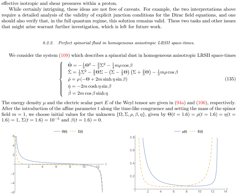
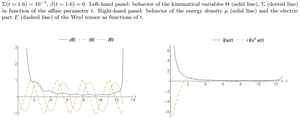
work page 1998
[23]

Covariant approach for perturbations of rotationally symmetric space-times

C. Clarkson, “Covariant approach for perturbations of rotationally symmetric space-times”,Phys Rev. D76, 104034 (2007)

work page 2007
[24]

Relativistic cosmology and large-scale structure

C. G. Tsagas, A. Challinor, R. Maartens, “Relativistic cosmology and large-scale structure”,Phys. Rep.465, 61 (2008)

work page 2008
[25]

Inhomogeneity and the foundations of concordance cosmology

C. Clarkson and R. Maartens, “Inhomogeneity and the foundations of concordance cosmology”,Class. Quant. Grav. 27, 124008 (2010)

work page 2010
[26]

Inhomogeneity effects in cosmology

G. F. R. Ellis, “Inhomogeneity effects in cosmology”,Class. Quant. Grav.28, 164001 (2011)

work page 2011
[27]

Nonlinear relativistic corrections to cosmological distances, redshift and gravitational lensing magnification: I. Key results

O. Umeh, C. Clarkson and R. Maartens, “Nonlinear relativistic corrections to cosmological distances, redshift and gravitational lensing magnification: I. Key results”,Class. Quant. Grav.31, 202001 (2014)

work page 2014
[28]

O. Umeh, C. Clarkson and R. Maartens, Nonlinear relativistic corrections to cosmological distances, redshift and gravitational lensing magnification: II. Derivation”,Class. Quant. Grav.31, 205001 (2014)

work page 2014
[29]

Covariant Tolman-Oppenheimer-Volkoff equations. I. The isotropic case

S. Carloni and D. Vernieri, “Covariant Tolman-Oppenheimer-Volkoff equations. I. The isotropic case”,Phys. Rev. D97, 124056 (2018)

work page 2018
[30]

Covariant Tolman-Oppenheimer-Volkoff equations. II. The anisotropic case

S. Carloni and D. Vernieri, “Covariant Tolman-Oppenheimer-Volkoff equations. II. The anisotropic case”,Phys. Rev. D97, 124057 (2018)

work page 2018
[31]

Two-fluid stellar objects in general relativity: The covariant formulation

N. F. Naidu, S. Carloni and P. Dunsby, “Two-fluid stellar objects in general relativity: The covariant formulation”, Phys. Rev. D104, 044014 (2021)

work page 2021
[32]

Anisotropic two-fluid stellar objects in general relativity

N. F. Naidu, S. Carloni and P. Dunsby, “Anisotropic two-fluid stellar objects in general relativity”,Phys. Rev. D 106, 124023 (2022)

work page 2022
[33]

Gauge invariant perturbations of static spatially compact LRS II space-times

P. Luz and S. Carloni, “Gauge invariant perturbations of static spatially compact LRS II space-times”,Class. Quant. Grav.41, 235012 (2024)

work page 2024
[34]

Noncomoving description of adiabatic radial perturbations of relativistic stars

P. Luz and S. Carloni, “Noncomoving description of adiabatic radial perturbations of relativistic stars”,Phys. Rev. D110, 084055 (2024)

work page 2024
[35]

Adiabatic radial perturbations of relativistic stars: Analytic solutions to an old problem

P. Luz and S. Carloni, “Adiabatic radial perturbations of relativistic stars: Analytic solutions to an old problem”, Phys. Rev. D110, 084054 (2024)

work page 2024
[36]

Gauge invariant perturbations of Scalar-Tensor Cosmologies: The Vacuum case

S. Carloni, P. K. S. Dunsby and C. Rubano, “Gauge invariant perturbations of Scalar-Tensor Cosmologies: The Vacuum case”,Phys. Rev. D74, 123513 (2006)

work page 2006
[37]

Derrick’s theorem in curved space-time

S. Carloni and J. L. Rosa, “Derrick’s theorem in curved space-time”,Phys. Rev. D100, 025014 (2019)

work page 2019
[38]

Introduction des param` etres relativistes de Cayley-Klein dans la repr´ esentation 27 hydrodynamique de l’´ equation de Dirac

G. Jakobi, G. Lochak, “Introduction des param` etres relativistes de Cayley-Klein dans la repr´ esentation 27 hydrodynamique de l’´ equation de Dirac”,Comp. Rend. Acad. Sci.243, 234 (1956)

work page 1956
[39]

Decomposition en param` etres de Clebsch de l’impulsion de Dirac et interpr´ etation physique de l’invariance de jauge des ´ equations de la M´ ecanique ondulatoire

G. Jakobi, G. Lochak, “Decomposition en param` etres de Clebsch de l’impulsion de Dirac et interpr´ etation physique de l’invariance de jauge des ´ equations de la M´ ecanique ondulatoire”,Comp. Rend. Acad. Sci.243, 357 (1956)

work page 1956
[40]

Relativistic Hydrodynamics Equivalent to the Dirac Equation

T. Takabayasi, “Relativistic Hydrodynamics Equivalent to the Dirac Equation”,Prog.Theor.Phys.13, 222 (1955)

work page 1955
[41]

Hydrodynamical Description of the Dirac Equation

T. Takabayasi, “Hydrodynamical Description of the Dirac Equation”,Nuovo Cimento3, 233 (1956)

work page 1956
[42]

Relativistic Hydrodynamics of the Dirac Matter

T. Takabayasi, “Relativistic Hydrodynamics of the Dirac Matter”,Prog. Theor. Phys. Supplement4, 1 (1957)

work page 1957
[43]

Dirac Theory in Hydrodynamic Form

Luca Fabbri, “Dirac Theory in Hydrodynamic Form”,Found. Phys.53, 54 (2023)

work page 2023
[44]

Polar form of Dirac fields: implementing symmetries via Lie derivative

L. Fabbri, S. Vignolo, R. Cianci, “Polar form of Dirac fields: implementing symmetries via Lie derivative”,Lett. Math. Phys.114, 21 (2024)

work page 2024
[45]

Dirac Fields in Hydrodynamic Form and their Thermodynamic Formulation

L. Fabbri, S. Vignolo, G. De Maria and S. Carloni, “Dirac Fields in Hydrodynamic Form and their Thermodynamic Formulation”, submitted for publication, [arXiv:2506.02608 [math-ph]]

work page arXiv
[46]

A covariant approach to the Dirac field in LRS space-times

S. Vignolo, G. De Maria, L. Fabbri and S. Carloni, “A covariant approach to the Dirac field in LRS space-times”, Class. Quantum Grav.42, 215013 (2025)

work page 2025
[47]

Dynamics of PressureFree Matter in General Relativity

G. F. R. Ellis, “Dynamics of PressureFree Matter in General Relativity”,J. Math. Phys.8, 1171 (1967)

work page 1967
[48]

Solutions of Einstein’s Equations for a Fluid Which Exhibit Local Rotational Symmetry

J. M. Stewart and G. F. R. Ellis, “Solutions of Einstein’s Equations for a Fluid Which Exhibit Local Rotational Symmetry”,J. Math. Phys.9, 1072 (1968)

work page 1968
[49]

A dynamical system formulation for inhomogeneous LRS-II spacetimes

S. Chakraborty, P. K. S. Dunsby, R. Goswami and A. Abebe, “A dynamical system formulation for inhomogeneous LRS-II spacetimes”,JCAP2024, 054 (2024)

work page 2024
[50]

S. W. Hawking and G. F. R. Ellis,The Large Scale Structure of Space-Time. Cambridge University Press, 1973

work page 1973
[51]

The pressure distribution inside the proton

Burkert, V. D., Elouadrhiri, L., Girod, F. X., “The pressure distribution inside the proton”,Nature557, 396 (2018)

work page 2018
[52]

Forces inside hadrons: pressure, surface tension, mechanical radius, and all that

Polyakov, M. V., Schweitzer, P., “Forces inside hadrons: pressure, surface tension, mechanical radius, and all that”,Int. J. Mod. Phys. A33, 1830025 (2018)

work page 2018
[53]

Pressure inside hadrons: criticism, conjectures, and all that

Lorc´ e, C., Schweitzer, P., “Pressure inside hadrons: criticism, conjectures, and all that”,Acta Phys. Polon. B56, 3–A17 (2025)

work page 2025
[54]

Revisiting the mechanical properties of the nucleon

Lorc´ e, C., Moutarde, H., Trawi´ nski, A. P., “Revisiting the mechanical properties of the nucleon”,Eur. Phys. J. C79, 89 (2019)

work page 2019
[55]

General relativistic boson stars,

F. E. Schunck and E. W. Mielke, “General relativistic boson stars,” Class. Quant. Grav.20(2003), R301-R356 doi:10.1088/0264-9381/20/20/201 [arXiv:0801.0307 [astro-ph]]. 28

work page doi:10.1088/0264-9381/20/20/201 2003