Recognition: 2 theorem links
· Lean TheoremError whitening: Why Gauss-Newton outperforms Newton
Pith reviewed 2026-05-13 02:04 UTC · model grok-4.3
The pith
Gauss-Newton descent whitens prediction errors by projecting onto the model's tangent space and replacing JJ^T with the identity, unlike Newton's method.
A machine-rendered reading of the paper's core claim, the machinery that carries it, and where it could break.
Core claim
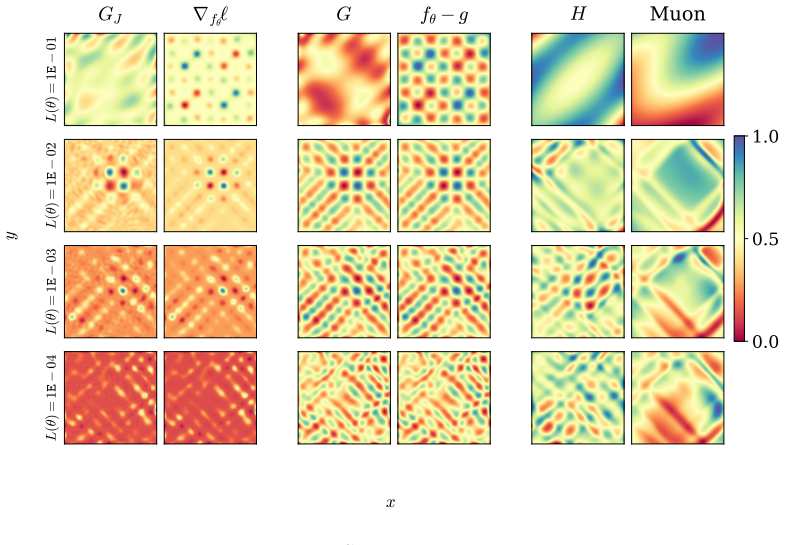
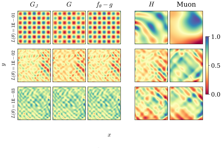
The generalized Gauss-Newton matrix projects the Newton direction in function space onto the model's tangent space, while a Jacobian-only variant projects the function space loss gradient onto the same tangent space. Both projections eliminate distortions from the model's parameterization by replacing JJ^T with the identity. This effect is called error whitening. Once the parameterization is removed, the prediction-target mismatch evolves according to dynamics dictated by the structure of the loss and the projection produced by the optimizer. Error whitening is a special property of Gauss-Newton descent that rigorously distinguishes it from Newton's method.
What carries the argument
The function-space projection performed by the generalized Gauss-Newton matrix onto the model's tangent space, which replaces the parameterization matrix JJ^T with the identity.
If this is right
- The mismatch between model predictions and targets evolves independently of the model's parameterization once the projection is applied.
- Gauss-Newton optimizers follow the theoretically predicted function-space dynamics in practice.
- Gauss-Newton descent outperforms Newton's method as well as Adam and Muon on supervised learning, physics-informed deep learning, and approximate dynamic programming tasks.
- After whitening, optimization dynamics are governed only by the chosen loss and the specific projection induced by the optimizer.
Where Pith is reading between the lines
- The same projection idea could be used to construct new first-order methods that inherit the whitening property without computing second derivatives.
- In overparameterized regimes where the tangent space is high-dimensional, the whitening effect may become even more pronounced and explain the practical success of Gauss-Newton-style updates.
- Design choices that preserve or destroy the tangent-space projection could be used to predict optimizer behavior on new loss functions before running large-scale experiments.
Load-bearing premise
The function-space projection analysis accurately captures the dominant dynamics of optimization without higher-order or discretization effects altering the JJ^T cancellation.
What would settle it
A controlled experiment in which the measured evolution of the prediction-target mismatch under Gauss-Newton deviates from the trajectory predicted by setting JJ^T to the identity in a simple non-least-squares loss.
Figures


read the original abstract
The Gauss-Newton matrix is widely viewed as a positive semidefinite approximation of the Hessian, yet mounting empirical evidence shows that Gauss-Newton descent outperforms Newton's method. We adopt a function space perspective to analyze this phenomenon. We show that the generalized Gauss-Newton (GGN) matrix projects the Newton direction in function space onto the model's tangent space, while a Jacobian-only variant obtained by applying the least squares Gauss-Newton matrix to non-least squares losses projects the function space loss gradient onto this same tangent space. Both projections eliminate distortions from the model's parameterization. Specifically, the evolution of the prediction-target mismatch depends on the model's parameterization through the matrix $JJ^\top$ where $J$ is the Jacobian of the model with respect to its parameters. The projections effectively replace $JJ^\top$ with the identity. We call this effect error whitening. Once the parameterization is removed, the prediction-target mismatch evolves according to dynamics dictated by the structure of the loss and the projection produced by the optimizer. Error whitening is a special property of Gauss-Newton descent that rigorously distinguishes it from Newton's method. We empirically demonstrate that Gauss-Newton optimizers follow the theoretically predicted function space dynamics and outperforms Newton's method, Adam, and Muon across case studies spanning supervised learning, physics-informed deep learning, and approximate dynamic programming.
Editorial analysis
A structured set of objections, weighed in public.
Referee Report
Summary. The paper claims that Gauss-Newton (GN) descent outperforms Newton's method because the generalized Gauss-Newton matrix projects the Newton direction (or loss gradient for a Jacobian-only variant) onto the model's tangent space in function space. This 'error whitening' effect replaces the parameterization-dependent JJ^T with the identity in the evolution of the prediction-target mismatch, so that dynamics depend only on loss structure and the projection. The analysis is supported by derivations and empirical trajectory matching showing GN superiority over Newton, Adam, and Muon in supervised learning, physics-informed networks, and approximate dynamic programming.
Significance. If the function-space projection view holds, the work supplies a principled distinction between GN and Newton that goes beyond the usual positive-semidefinite approximation narrative, potentially informing second-order optimizer design in deep learning. The empirical demonstrations of predicted dynamics are a concrete strength.
major comments (2)
- The central claim that error whitening 'rigorously distinguishes' GN from Newton rests on the projection analysis capturing dominant dynamics. The manuscript should explicitly bound or test the effect of higher-order terms in the model expansion and finite-step discretization on the JJ^T cancellation, especially in the finite-width non-convex regimes of the case studies (as the weakest assumption in the provided analysis). Without this, the distinction may not transfer as stated.
- Handling of non-least-squares losses via the Jacobian-only variant: the abstract sketches the projection but the manuscript lacks visible details on proof completeness for this case; a self-contained derivation or counter-example would be needed to support the general claim.
minor comments (2)
- Notation: the early definition and consistent use of J (Jacobian) and JJ^T should be clarified with a small example to aid readers new to the function-space perspective.
- Empirical sections: adding error bars or multiple random seeds to the trajectory-matching plots would improve readability and statistical clarity without altering the core results.
Simulated Author's Rebuttal
We thank the referee for the constructive and detailed feedback. The comments highlight important aspects of the analysis that we have addressed through revisions to improve clarity and rigor.
read point-by-point responses
-
Referee: The central claim that error whitening 'rigorously distinguishes' GN from Newton rests on the projection analysis capturing dominant dynamics. The manuscript should explicitly bound or test the effect of higher-order terms in the model expansion and finite-step discretization on the JJ^T cancellation, especially in the finite-width non-convex regimes of the case studies (as the weakest assumption in the provided analysis). Without this, the distinction may not transfer as stated.
Authors: We agree that the projection analysis relies on a first-order model expansion and that higher-order terms, along with finite discretization effects, could in principle affect the exact cancellation of JJ^T. Our empirical trajectory-matching experiments already demonstrate close agreement with the predicted dynamics in the finite-width non-convex settings of the case studies, suggesting the leading-order effect remains dominant. In the revision we have added a dedicated subsection that derives the leading remainder term in the Taylor expansion and reports additional numerical tests that vary step size and measure the resulting deviation from the idealized linear dynamics. While a fully general, tight bound for arbitrary non-convex finite-width networks lies beyond the scope of the present work, these additions make the domain of validity of the distinction explicit. revision: partial
-
Referee: Handling of non-least-squares losses via the Jacobian-only variant: the abstract sketches the projection but the manuscript lacks visible details on proof completeness for this case; a self-contained derivation or counter-example would be needed to support the general claim.
Authors: We thank the referee for noting the need for greater detail on the Jacobian-only variant. The algebraic steps showing that the least-squares GGN applied to a general loss gradient yields the tangent-space projection (and thereby replaces JJ^T with the identity) were present but not fully expanded. The revised manuscript now contains a self-contained derivation in the main text that walks through each matrix identity and the resulting evolution equation for the prediction-target mismatch. Because the derivation is algebraic and holds under the stated assumptions on the loss and Jacobian, a counter-example is not required; we have added a short remark clarifying the assumptions and their implications for non-least-squares objectives. revision: yes
Circularity Check
No circularity: function-space projection analysis is self-contained linear algebra
full rationale
The derivation begins from the standard definitions of the Newton and Gauss-Newton updates, applies the function-space gradient and Jacobian projection operators, and shows algebraically that the GGN step replaces JJ^T by the identity in the evolution equation for the prediction-target mismatch. This replacement follows directly from the matrix forms of the two optimizers and does not rely on any fitted parameter, self-citation chain, or ansatz imported from prior work by the same authors. The subsequent claim that this constitutes 'error whitening' is a naming of the derived identity rather than a redefinition that forces the result. Empirical sections compare observed trajectories to the predicted dynamics but do not feed fitted quantities back into the theoretical statements. The analysis therefore remains independent of its own outputs.
Axiom & Free-Parameter Ledger
axioms (2)
- domain assumption The local behavior of the model is captured by its Jacobian J, and updates act in the tangent space spanned by its columns.
- domain assumption The evolution of the prediction-target mismatch is governed by the composition of the loss gradient with the model Jacobian.
invented entities (1)
-
error whitening
no independent evidence
Lean theorems connected to this paper
-
IndisputableMonolith/Cost/FunctionalEquation.leanwashburn_uniqueness_aczel unclear?
unclearRelation between the paper passage and the cited Recognition theorem.
The projections effectively replace JJ^T with the identity. We call this effect error whitening... Once the parameterization is removed, the prediction-target mismatch evolves according to dynamics dictated by the structure of the loss
-
IndisputableMonolith/Foundation/AlphaCoordinateFixation.leancostAlphaLog_fourth_deriv_at_zero unclear?
unclearRelation between the paper passage and the cited Recognition theorem.
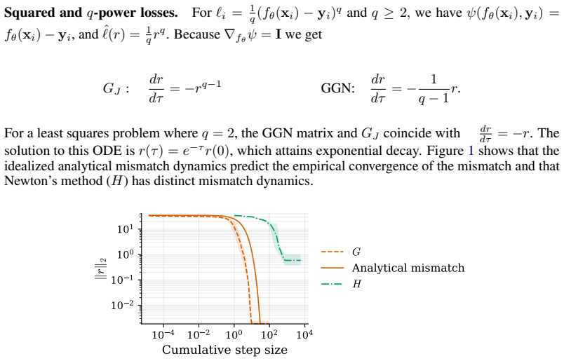
GJ : dr/dτ = -r ... solution r(τ)=e^{-τ} r(0)
What do these tags mean?
- matches
- The paper's claim is directly supported by a theorem in the formal canon.
- supports
- The theorem supports part of the paper's argument, but the paper may add assumptions or extra steps.
- extends
- The paper goes beyond the formal theorem; the theorem is a base layer rather than the whole result.
- uses
- The paper appears to rely on the theorem as machinery.
- contradicts
- The paper's claim conflicts with a theorem or certificate in the canon.
- unclear
- Pith found a possible connection, but the passage is too broad, indirect, or ambiguous to say the theorem truly supports the claim.
Reference graph
Works this paper leans on
-
[1]
The Potential of Second-Order Optimization for LLMs: A Study with Full Gauss-Newton
Natalie Abreu, Nikhil Vyas, Sham Kakade, and Depen Morwani. The potential of second-order optimization for llms: A study with full gauss-newton.arXiv preprint arXiv:2510.09378, 2025
work page internal anchor Pith review Pith/arXiv arXiv 2025
-
[2]
arXiv preprint arXiv:2002.09018 , year=
Rohan Anil, Vineet Gupta, Tomer Koren, Kevin Regan, and Yoram Singer. Scalable second order optimization for deep learning.arXiv preprint arXiv:2002.09018, 2021
-
[3]
Bellemare, Will Dabney, and Mark Rowland.Distributional Reinforcement Learning
Marc G. Bellemare, Will Dabney, and Mark Rowland.Distributional Reinforcement Learning. Adaptive Computation and Machine Learning. The MIT Press, Cambridge London, 2023
work page 2023
-
[4]
Dimitri Bertsekas.Dynamic Programming and Optimal Control: Volume I, volume 4. Athena scientific, 2012
work page 2012
-
[5]
Dimitri Bertsekas.Lessons from AlphaZero for Optimal, Model Predictive, and Adaptive Control. Athena Scientific, 2022
work page 2022
-
[6]
Dimitri Bertsekas and John N Tsitsiklis.Neuro-Dynamic Programming. Athena Scientific, 1996
work page 1996
-
[7]
Near-optimal sketchy natural gradients for physics-informed neural networks
Maricela Best Mckay, Avleen Kaur, Chen Greif, and Brian Wetton. Near-optimal sketchy natural gradients for physics-informed neural networks. InForty-Second International Conference on Machine Learning, 2025
work page 2025
- [8]
-
[9]
JAX: composable transformations of Python+NumPy programs, 2018
James Bradbury, Roy Frostig, Peter Hawkins, Matthew James Johnson, Yash Katariya, Chris Leary, Dougal Maclaurin, George Necula, Adam Paszke, Jake VanderPlas, Skye Wanderman- Milne, and Qiao Zhang. JAX: composable transformations of Python+NumPy programs, 2018
work page 2018
-
[10]
Pei Chen. Hessian Matrix vs. Gauss–Newton Hessian matrix.SIAM Journal on Numerical Analysis, 49(4):1417–1435, 2011
work page 2011
-
[11]
Yann N Dauphin, Razvan Pascanu, Caglar Gulcehre, Kyunghyun Cho, Surya Ganguli, and Yoshua Bengio. Identifying and attacking the saddle point problem in high-dimensional non- convex optimization.Advances in neural information processing systems, 27, 2014
work page 2014
-
[12]
Arka Daw, Jie Bu, Sifan Wang, Paris Perdikaris, and Anuj Karpatne. Mitigating propagation failures in physics-informed neural networks using retain-resample-release (r3) sampling. In Proceedings of the 40th International Conference on Machine Learning, pages 7264–7302, 2023
work page 2023
-
[13]
Suchuan Dong and Naxian Ni. A method for representing periodic functions and enforcing exactly periodic boundary conditions with deep neural networks.Journal of Computational Physics, 435:110242, 2021
work page 2021
-
[14]
Ján Drgo ˇna, Karol Kiš, Aaron Tuor, Draguna Vrabie, and Martin Klau ˇco. Differentiable predictive control: Deep learning alternative to explicit model predictive control for unknown nonlinear systems.Journal of Process Control, 116:80–92, 2022. 10
work page 2022
-
[15]
NeuroMANCER: Neural Modules with Adaptive Nonlinear Constraints and Efficient Regularizations
Jan Drgona, Aaron Tuor, James Koch, Madelyn Shapiro, Bruno Jacob, and Draguna Vra- bie. NeuroMANCER: Neural Modules with Adaptive Nonlinear Constraints and Efficient Regularizations. 2023
work page 2023
-
[16]
Roger Fletcher.Practical methods of optimization. John Wiley & Sons, 2013
work page 2013
-
[17]
A stable whitening optimizer for efficient neural network training
Kevin Frans, Sergey Levine, and Pieter Abbeel. A stable whitening optimizer for efficient neural network training. InThe Thirty-ninth Annual Conference on Neural Information Processing Systems
-
[18]
Addressing function approximation error in actor-critic methods
Scott Fujimoto, Herke van Hoof, and David Meger. Addressing function approximation error in actor-critic methods. InProceedings of the 35th International Conference on Machine Learning, volume 80 ofProceedings of Machine Learning Research, pages 1587–1596. PMLR, 2018
work page 2018
-
[19]
Carnegie Mellon University, 1999
Geoffrey J Gordon.Approximate Solutions to Markov Decision Processes. Carnegie Mellon University, 1999
work page 1999
-
[20]
Leonardo Ferreira Guilhoto and Paris Perdikaris. Deep learning alternatives of the kolmogorov superposition theorem.arXiv preprint arXiv:2410.01990, 2024
-
[21]
Shampoo: Preconditioned stochastic tensor optimization
Vineet Gupta, Tomer Koren, and Yoram Singer. Shampoo: Preconditioned stochastic tensor optimization. InProceedings of the 35th International Conference on Machine Learning, volume 80 ofProceedings of Machine Learning Research, pages 1842–1850. PMLR, 2018
work page 2018
-
[22]
Soft actor-critic: Off-policy maximum entropy deep reinforcement learning with a stochastic actor
Tuomas Haarnoja, Aurick Zhou, Pieter Abbeel, and Sergey Levine. Soft actor-critic: Off-policy maximum entropy deep reinforcement learning with a stochastic actor. InProceedings of the 35th International Conference on Machine Learning, volume 80 ofProceedings of Machine Learning Research, pages 1861–1870. PMLR, 2018
work page 2018
-
[23]
Double Q-learning.Advances in neural information processing systems, 23, 2010
Hado Hasselt. Double Q-learning.Advances in neural information processing systems, 23, 2010
work page 2010
-
[24]
Rainbow: Combining Improvements in Deep Reinforcement Learning, 2017
Matteo Hessel, Joseph Modayil, Hado van Hasselt, Tom Schaul, Georg Ostrovski, Will Dab- ney, Dan Horgan, Bilal Piot, Mohammad Azar, and David Silver. Rainbow: Combining Improvements in Deep Reinforcement Learning, 2017
work page 2017
-
[25]
The 37 implementation details of proximal policy optimization
Shengyi Huang, Rousslan Fernand Julien Dossa, Antonin Raffin, Anssi Kanervisto, and Weixun Wang. The 37 implementation details of proximal policy optimization. InICLR Blog Track, 2022
work page 2022
-
[26]
Anas Jnini, Flavio Vella, and Marius Zeinhofer. Gauss-newton natural gradient descent for physics-informed computational fluid dynamics.Computers & Fluids, page 106955, 2025
work page 2025
-
[27]
Ryo Karakida, Shotaro Akaho, and Shun-ichi Amari. Pathological spectra of the fisher informa- tion metric and its variants in deep neural networks.Neural Computation, 33(8):2274–2307, 2021
work page 2021
-
[28]
Adam: A Method for Stochastic Optimization
Diederik P Kingma and Jimmy Ba. Adam: A method for stochastic optimization.arXiv preprint arXiv:1412.6980, 2014
work page internal anchor Pith review Pith/arXiv arXiv 2014
-
[29]
Aditi Krishnapriyan, Amir Gholami, Shandian Zhe, Robert Kirby, and Michael W Mahoney. Characterizing possible failure modes in physics-informed neural networks.Advances in neural information processing systems, 34:26548–26560, 2021
work page 2021
-
[30]
Tim Large, Yang Liu, Minyoung Huh, Hyojin Bahng, Phillip Isola, and Jeremy Bernstein. Scalable optimization in the modular norm.Advances in Neural Information Processing Systems, 37:73501–73548, 2024
work page 2024
-
[31]
Yann LeCun, Léon Bottou, Yoshua Bengio, and Patrick Haffner. Gradient-based learning applied to document recognition.Proceedings of the IEEE, 86(11):2278–2324, 1998
work page 1998
-
[32]
Yann LeCun, Léon Bottou, Yoshua Bengio, and Patrick Haffner. Gradient-based learning applied to document recognition.Proceedings of the IEEE, 86(11):2278–2324, 2002. 11
work page 2002
-
[33]
Timothy P. Lillicrap, Jonathan J. Hunt, Alexander Pritzel, Nicolas Heess, Tom Erez, Yuval Tassa, David Silver, and Daan Wierstra. Continuous control with deep reinforcement learning. 2015
work page 2015
-
[34]
Carnegie Mellon University, 1992
Long-Ji Lin.Reinforcement Learning for Robots Using Neural Networks. Carnegie Mellon University, 1992
work page 1992
-
[35]
Dong C Liu and Jorge Nocedal. On the limited memory BFGS method for large scale optimiza- tion.Mathematical programming, 45(1):503–528, 1989
work page 1989
-
[36]
Decoupled weight decay regularization
Ilya Loshchilov and Frank Hutter. Decoupled weight decay regularization. InInternational Conference on Learning Representations, 2019
work page 2019
-
[37]
Understanding SOAP from the perspective of gradient whitening.arXiv preprint arXiv:2509.22938, 2025
Yanqing Lu, Letao Wang, and Jinbo Liu. Understanding SOAP from the perspective of gradient whitening.arXiv preprint arXiv:2509.22938, 2025
-
[38]
James Martens. New insights and perspectives on the natural gradient method.Journal of Machine Learning Research, 21(146):1–76, 2020
work page 2020
-
[39]
Optimizing neural networks with kronecker-factored approx- imate curvature
James Martens and Roger Grosse. Optimizing neural networks with kronecker-factored approx- imate curvature. InInternational conference on machine learning, pages 2408–2417. PMLR, 2015
work page 2015
-
[40]
Asynchronous methods for deep reinforcement learning.arXiv preprint arXiv:1602.01783,
V olodymyr Mnih, Adrià Puigdomènech Badia, Mehdi Mirza, Alex Graves, Timothy P. Lilli- crap, Tim Harley, David Silver, and Koray Kavukcuoglu. Asynchronous Methods for Deep Reinforcement Learning.arXiv:1602.01783 [cs], 2016
-
[41]
Playing Atari with Deep Reinforcement Learning, 2013
V olodymyr Mnih, Koray Kavukcuoglu, David Silver, Alex Graves, Ioannis Antonoglou, Daan Wierstra, and Martin Riedmiller. Playing Atari with Deep Reinforcement Learning, 2013
work page 2013
-
[42]
A new perspective on shampoo’s preconditioner
Depen Morwani, Itai Shapira, Nikhil Vyas, Eran Malach, Sham Kakade, and Lucas Janson. A new perspective on shampoo’s preconditioner. InInternational Conference on Learning Representations, 2025
work page 2025
-
[43]
Achieving high accuracy with PINNs via energy natural gradient descent
Johannes Müller and Marius Zeinhofer. Achieving high accuracy with PINNs via energy natural gradient descent. InInternational Conference on Machine Learning, pages 25471–25485. PMLR, 2023
work page 2023
-
[44]
Jorge Nocedal and Stephen J Wright.Numerical optimization. Springer, 2006
work page 2006
-
[45]
Adam Paszke, Sam Gross, Francisco Massa, Adam Lerer, James Bradbury, Gregory Chanan, Trevor Killeen, Zeming Lin, Natalia Gimelshein, Luca Antiga, et al. PyTorch: An imperative style, high-performance deep learning library.Advances in neural information processing systems, 32, 2019
work page 2019
-
[46]
Powell.Approximate Dynamic Programming: Solving the Curses of Dimensionality
Warren B. Powell.Approximate Dynamic Programming: Solving the Curses of Dimensionality. Wiley Series in Probability and Statistics. Wiley, Hoboken, N.J, 2nd ed edition, 2011
work page 2011
- [47]
-
[48]
Martin Riedmiller. Neural Fitted Q Iteration – First Experiences with a Data Efficient Neural Reinforcement Learning Method. InMachine Learning: ECML 2005, volume 3720, pages 317–328. Springer Berlin Heidelberg, Berlin, Heidelberg, 2005
work page 2005
-
[49]
Rohrhofer, Stefan Posch, Clemens Gößnitzer, and Bernhard C Geiger
Franz M. Rohrhofer, Stefan Posch, Clemens Gößnitzer, and Bernhard C Geiger. On the role of fixed points of dynamical systems in training physics-informed neural networks.Transactions on Machine Learning Research, 2022
work page 2022
-
[50]
Tom Schaul, John Quan, Ioannis Antonoglou, and David Silver. Prioritized experience replay. arXiv preprint arXiv:1511.05952, 2015. 12
work page Pith review arXiv 2015
-
[51]
Trust region policy optimization
John Schulman, Sergey Levine, Pieter Abbeel, Michael Jordan, and Philipp Moritz. Trust region policy optimization. InProceedings of the 32nd International Conference on Machine Learning, volume 37 ofProceedings of Machine Learning Research, pages 1889–1897, Lille, France, 2015. PMLR
work page 2015
-
[52]
Proximal policy optimization algorithms
John Schulman, Filip Wolski, Prafulla Dhariwal, Alec Radford, and Oleg Klimov. Proximal policy optimization algorithms. 2017
work page 2017
-
[53]
Weijie Su, Stephen Boyd, and Emmanuel J Candes. A differential equation for modeling nesterov’s accelerated gradient method: Theory and insights.Journal of Machine Learning Research, 17(153):1–43, 2016
work page 2016
-
[54]
Richard S. Sutton. Learning to predict by the methods of temporal differences.Machine Learning, 3(1):9–44, 1988
work page 1988
-
[55]
Richard S. Sutton and Andrew G. Barto.Reinforcement Learning: An Introduction. Adaptive Computation and Machine Learning Series. The MIT Press, Cambridge, Massachusetts, second edition edition, 2018
work page 2018
-
[56]
Russ Tedrake.Underactuated Robotics. 2023
work page 2023
-
[57]
SOAP: Improving and stabilizing shampoo using adam
Nikhil Vyas, Depen Morwani, Rosie Zhao, Mujin Kwun, Itai Shapira, David Brandfonbrener, Lucas Janson, and Sham Kakade. SOAP: Improving and stabilizing shampoo using adam. In International Conference on Learning Representations, 2025
work page 2025
-
[58]
Gradient alignment in physics- informed neural networks: a second-order optimization perspective
Sifan Wang, Ananyae Kumar Bhartari, Bowen Li, and Paris Perdikaris. Gradient alignment in physics-informed neural networks: A second-order optimization perspective.arXiv preprint arXiv:2502.00604, 2025
-
[59]
Sifan Wang, Bowen Li, Yuhan Chen, and Paris Perdikaris. Piratenets: Physics-informed deep learning with residual adaptive networks.Journal of Machine Learning Research, 25(402):1–51, 2024
work page 2024
-
[60]
Respecting causality is all you need for training physics-informed neural networks
Sifan Wang, Shyam Sankaran, and Paris Perdikaris. Respecting causality is all you need for training physics-informed neural networks.arXiv preprint arXiv:2203.07404, 2022
-
[61]
An expert’s guide to training physics-informed neural networks.arXiv preprint arXiv:2308.08468, 2023
Sifan Wang, Shyam Sankaran, Hanwen Wang, and Paris Perdikaris. An expert’s guide to training physics-informed neural networks.arXiv preprint arXiv:2308.08468, 2023
-
[62]
Sifan Wang, Yujun Teng, and Paris Perdikaris. Understanding and mitigating gradient flow pathologies in physics-informed neural networks.SIAM Journal on Scientific Computing, 43(5):A3055–A3081, January 2021
work page 2021
-
[63]
Sifan Wang, Xinling Yu, and Paris Perdikaris. When and why PINNs fail to train: A neural tangent kernel perspective.Journal of Computational Physics, 449:110768, January 2022
work page 2022
-
[64]
Dueling network architectures for deep reinforcement learning
Ziyu Wang, Tom Schaul, Matteo Hessel, Hado Hasselt, Marc Lanctot, and Nando Freitas. Dueling network architectures for deep reinforcement learning. InInternational Conference on Machine Learning, pages 1995–2003. PMLR, 2016
work page 1995
-
[65]
Jian Cheng Wong, Chin Chun Ooi, Abhishek Gupta, and Yew-Soon Ong. Learning in sinusoidal spaces with physics-informed neural networks.IEEE Transactions on Artificial Intelligence, 5(3):985–1000, 2022
work page 2022
-
[66]
Principal whitened gradient for information geometry
Zhirong Yang and Jorma Laaksonen. Principal whitened gradient for information geometry. Neural Networks, 21(2-3):232–240, 2008. 13 A Identities and useful calculations Lemma A.1.For any matrix M∈R m×n with rank r, (M ⊤M) †M ⊤ =M †. This is a standard well known result included here simply for completeness. Proof. Consider the singular value decomposition ...
work page 2008
-
[67]
0σ −2 r | {z } r×rnonzero block 0|{z} r×(n−r) 0|{z} (n−r)×r 0|{z} (n−r)×(n−r) σ1 0· · ·0 0σ 2
-
[68]
0σ r | {z } r×rnonzero block 0|{z} r×(m−r) 0|{z} (n−r)×r 0|{z} (n−r)×(m−r) U ⊤ =V 1/σ1 0· · ·0 0 1/σ 2
-
[69]
0 1/σ r | {z } r×rnonzero block 0|{z} r×(m−r) 0|{z} (n−r)×r 0|{z} (n−r)×(m−r) U ⊤ =VΣ †U ⊤ =M †. 14 Corollary A.2. M M† =UΣV ⊤VΣ †U ⊤ =UΣΣ †U ⊤ =U σ1 0· · ·0 0σ 2
-
[70]
0σ r | {z } r×rnonzero block 0|{z} r×(n−r) 0|{z} (m−r)×r 0|{z} (m−r)×(n−r) 1/σ1 0· · ·0 0 1/σ 2
-
[71]
0 1/σ r | {z } r×rnonzero block 0|{z} r×(m−r) 0|{z} (n−r)×r 0|{z} (n−r)×(m−r) U ⊤ =U 1 0· · ·0 0 1
-
[72]
0 1 | {z } r×rIdentity block 0|{z} r×(m−r) 0|{z} (m−r)×r 0|{z} (m−r)×(m−r) U ⊤ = Ur|{z} m×r 0|{z} (m)×(m−r) U ⊤ = rX i=1 U[:,i]U ⊤ [:,i]. Proposition A.3.Equivalence of writing (G)†∇θL(θ) as a product of summed matrices vs as stacked matrix vector products, i.e. J 1 d dX i=1 J ⊤ i ∇2 fθ ℓiJi !† 1 d dX i=1 J ⊤ i ∇fθ ℓi ! =J J ⊤∇2 fθ ℓ(...
-
[73]
∇2 fθ ℓd −1/2 ∇fθ ℓd | {z } dk×1
0 1 | {z } r×rIdentity block 0|{z} r×(dk−r) 0|{z} (dk−r)×r 0|{z} (dk−r)×(dk−r) U ⊤ 1 d ∇2 fθ ℓ1 −1/2 ∇fθ ℓ1 ... ∇2 fθ ℓd −1/2 ∇fθ ℓd | {z } dk×1 . So, U ⊤ ∇2 fθ ℓ(fθ) 1/2 dfθ dτ =− Ir 0 0 0 U ⊤ 1 d ∇2 fθ ℓ1 −1/2 ∇fθ ℓ1 ... ∇2 fθ ℓd −1/2 ∇fθ ℓd | {z } dk×1 . 16 ∇2 fθ ℓ(fθ) −1 ∇fθ ℓ(fθ) = 1 d ...
-
[74]
It is the cosine of the angle between v and the subspace Im(J)
This tells us how much of v is in Im(J). It is the cosine of the angle between v and the subspace Im(J). If the ratio is 1, then all of v is in the subspace; if it is 0, then none ofvis in the subspace. A similar computation yields the reachability of the GGN. Here, we need to compute in the weighted norm 1 d J ⊤HℓJ v Hℓ : 1 d J(J ⊤HℓJ) †J ⊤v 2 Hℓ = X i d...
-
[75]
Gauss–Newton descent corresponds to the Newton update direction in function space, restricted to directions reachable through parameter updates
-
[76]
Moreover, this direction is the unique minimizer of min v∈Im(∇θfθ) 1 2 v+H −1 ℓ ∇fθ ℓ(fθ) 2 Hℓ . Proof. Let Ji :=∇ θfθ(xi) and J= [ J1, . . . , J d]⊤ | {z } dk×p denote the vectorized matrix containing each sample Jacobian. Note that the vectorized Hessian ∇2 fθ ℓ(fθ) | {z } dk×dk = 1 d ∇2 fθ ℓ1 | {z } k×k 0· · ·0 0∇ 2 fθ ℓ2 . . . ... ... . ....
work page 2000
discussion (0)
Sign in with ORCID, Apple, or X to comment. Anyone can read and Pith papers without signing in.