Recognition: no theorem link
The unified transform for Burgers' equation: Application to unsaturated flow in finite interval
Pith reviewed 2026-05-13 05:47 UTC · model grok-4.3
The pith
The Unified Transform Method supplies an explicit integral representation for solutions of the linearized Burgers equation on a finite interval.
A machine-rendered reading of the paper's core claim, the machinery that carries it, and where it could break.
Core claim
The Unified Transform Method yields an explicit integral representation of the solution to the diffusion equation on a finite interval with mixed boundary conditions that arises from linearizing Burgers' equation for modeling unsaturated flow.
What carries the argument
The Unified Transform Method, which derives a global relation from the PDE and boundary conditions to construct an explicit integral representation of the solution.
If this is right
- The method allows direct computation of water content profiles in finite soil columns without relying on series expansions.
- Improved numerical stability facilitates more reliable simulations of infiltration processes over longer times or with sharper gradients.
- Applications in hydrology can leverage this for better handling of boundary conditions in bounded domains.
Where Pith is reading between the lines
- Similar integral representations could apply to other nonlinear PDEs in hydrology after suitable transformations.
- Testing the method on problems with variable diffusivity would reveal its robustness beyond the constant case assumed here.
- Integration with existing hydrological software might improve efficiency in predicting soil moisture dynamics.
Load-bearing premise
The assumptions that diffusivity is constant and hydraulic conductivity depends quadratically on water content, which permit the exact reduction of Richards' equation to Burgers' equation and its linearization.
What would settle it
Numerical tests on the finite interval problem where the integral representation diverges or fails to match the Fourier series solution for chosen initial and boundary data.
Figures


read the original abstract
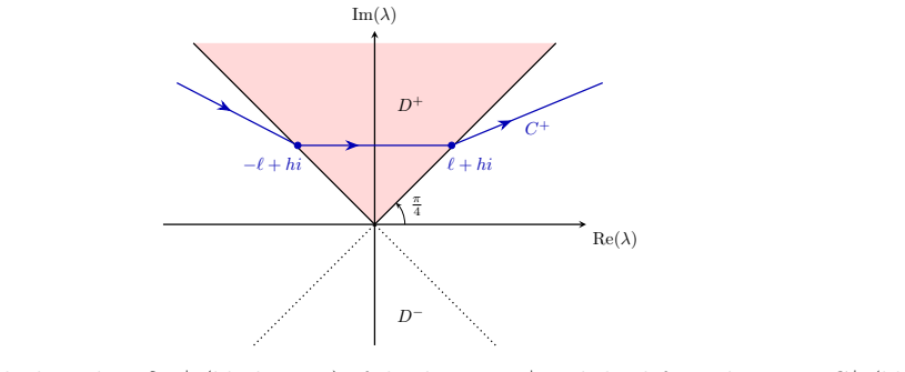
In this paper, we focus on one-dimensional vertical infiltration, assuming constant diffusivity and a quadratic relationship between hydraulic conductivity and water content. Under these assumptions, Richards' equation reduces to Burgers' equation, which we then linearize via the Hopf-Cole transformation. This turns the initial boundary value problem into a diffusion equation on a finite interval with mixed boundary conditions. To solve it, we use the Unified Transform Method (also known as the Fokas method). This approach gives an explicit integral representation of the solution, and when evaluated numerically, the results match classical Fourier series solutions exactly, but with better convergence and stability. Two examples from hydrological applications are examined.
Editorial analysis
A structured set of objections, weighed in public.
Referee Report
Summary. The manuscript applies the Unified Transform Method (Fokas method) to the heat equation obtained after Hopf-Cole linearization of Burgers' equation, which arises from Richards' equation for one-dimensional vertical infiltration under the assumptions of constant diffusivity and quadratic hydraulic conductivity. It derives an explicit integral representation for the solution on a finite interval subject to mixed boundary conditions and presents numerical evaluations that are asserted to match classical Fourier-series solutions exactly while showing improved convergence and stability. Two hydrological application examples are examined.
Significance. If the derivation and numerical claims hold, the work supplies an alternative explicit representation for linearized infiltration problems that may avoid Gibbs phenomena or slow decay associated with eigenfunction expansions, offering potential advantages for stable long-time simulations in hydrology. The approach aligns with known strengths of contour-integral methods for linear IBVPs and could extend to related nonlinear diffusion models once the linearization assumptions are satisfied.
major comments (2)
- [§3] §3, Eq. (3.8): the global relation is stated but the explicit elimination of the unknown boundary values (arising from the mixed Dirichlet-Neumann conditions after Hopf-Cole) is not carried out in detail; without this step the claimed explicit integral representation cannot be verified independently.
- [§4.2] §4.2, Figure 3: the reported numerical agreement with the Fourier solution is shown only via overlaid plots; no L²-error tables, convergence rates versus number of quadrature points, or contour-deformation parameters are supplied, so the asserted superiority in convergence and stability remains unquantified.
minor comments (2)
- [Abstract] The abstract and §1 state that the numerical results 'match exactly'; this should be rephrased as 'agree to machine precision' to reflect floating-point evaluation of the contour integrals.
- [§2] Notation for the transformed boundary functions (e.g., the functions appearing in the global relation) is introduced without a dedicated table or list of symbols, reducing readability.
Simulated Author's Rebuttal
We thank the referee for the careful reading and constructive comments on our manuscript. We address each major comment below and indicate the revisions planned to improve clarity and support for the claims.
read point-by-point responses
-
Referee: [§3] §3, Eq. (3.8): the global relation is stated but the explicit elimination of the unknown boundary values (arising from the mixed Dirichlet-Neumann conditions after Hopf-Cole) is not carried out in detail; without this step the claimed explicit integral representation cannot be verified independently.
Authors: We appreciate this observation. While the global relation and its role in the unified transform are presented in Section 3, we agree that the elimination of the unknown boundary values for the mixed conditions could be shown with additional explicit steps to facilitate independent verification. In the revised manuscript we will expand this derivation, inserting the intermediate algebraic manipulations that solve for the unknown transforms and yield the final contour-integral formula. revision: yes
-
Referee: [§4.2] §4.2, Figure 3: the reported numerical agreement with the Fourier solution is shown only via overlaid plots; no L²-error tables, convergence rates versus number of quadrature points, or contour-deformation parameters are supplied, so the asserted superiority in convergence and stability remains unquantified.
Authors: We agree that quantitative evidence is needed to substantiate the asserted advantages in convergence and stability. In the revised version we will add L²-error tables for representative test cases, report observed convergence rates as a function of quadrature points, and document the contour-deformation parameters used in the numerical evaluations of the integral representation. revision: yes
Circularity Check
No significant circularity identified
full rationale
The paper reduces Richards' equation to Burgers' equation under constant diffusivity and quadratic conductivity assumptions, applies the Hopf-Cole transformation to obtain the linear heat equation on a finite interval with mixed boundary conditions, and then invokes the established Unified Transform Method (Fokas method) to derive an explicit contour-integral representation. This representation is shown to agree numerically with the classical Fourier-series solution of the identical IBVP, which is expected once both methods correctly enforce the global relation and eliminate unknown boundary values. No step reduces by definition to its own inputs, no fitted parameter is relabeled as a prediction, and no load-bearing premise rests on a self-citation chain; the derivation is self-contained against the external benchmark of the standard eigenfunction expansion.
Axiom & Free-Parameter Ledger
axioms (2)
- standard math Hopf-Cole transformation converts Burgers' equation into a linear diffusion equation
- domain assumption Constant diffusivity and quadratic hydraulic conductivity-water content relation reduce Richards' equation to Burgers' equation
Reference graph
Works this paper leans on
-
[1]
I. Argyrokastritis, K. Kalimeris, and L. Mindrinos. An analytical solution for vertical infiltration in homogeneous bounded profiles.European Journal of Soil Science, 75(4):e13547, 2024
work page 2024
-
[2]
H. Basha. Burgers’ equation: A general nonlinear solution of infiltration and redistribution. Water Resources Research, 38(11):29–1, 2002
work page 2002
-
[3]
C. Braester. Moisture variation at the soil surface and the advance of the wetting front during infiltration at constant flux.Water Resources Research, 9(3):687–694, 1973. 9 Figure 4: Convergence of the series solution to the analytical one (blue curve) fort= 40 min for the setup of the first example. Figure 5: Example 1: The three-dimensional visualizati...
work page 1973
-
[4]
J. M. Burgers. A mathematical model illustrating the theory of turbulence.Advances in applied mechanics, 1:171–199, 1948
work page 1948
-
[5]
H. S. Carslaw and J. C. Jaeger.Conduction of heat in solids. Oxford University Press, London, 1959
work page 1959
-
[6]
A. Chatziafratis, A. Fokas, and K. Kalimeris. The fokas method for evolution partial differential equations.Partial Differential Equations in Applied Mathematics, 14:101144, 2025
work page 2025
-
[7]
A. Chatziafratis and D. Mantzavinos. Boundary behavior for the heat equation on the half-line. Mathematical Methods in the Applied Sciences, 45(12):7364–7393, 2022
work page 2022
-
[8]
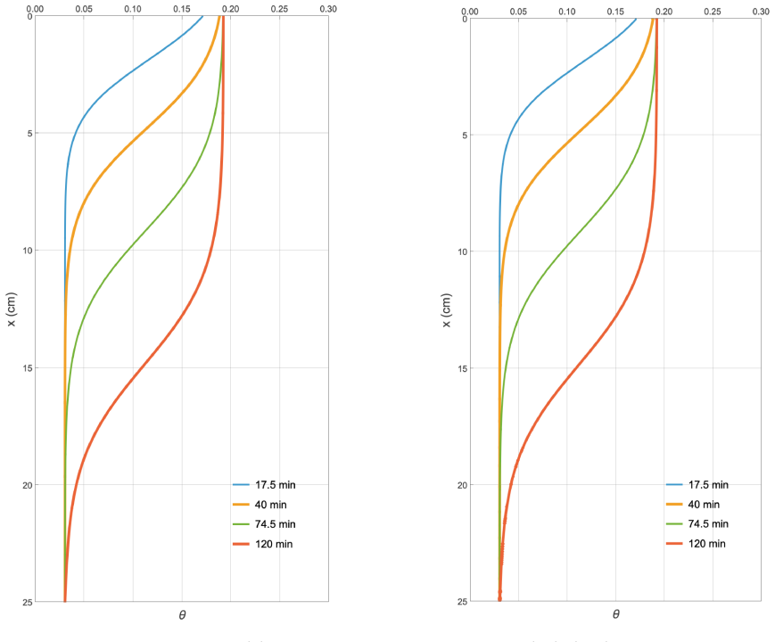
B. E. Clothier, J. H. Knight, and I. White. Burgers’ equation: Application to field constant-flux infiltration.Soil Science, 132(4):255–261, 1981. 10 Figure 6: The water contentθ(6) using the analytical solution (14) (left) and the Fourier series solution, see [16], (right) for the setup of the second example
work page 1981
-
[9]
F. P. J. De Barros, M. J. Colbrook, and A. S. Fokas. A hybrid analytical-numerical method for solving advection-dispersion problems on a half-line.International Journal of Heat and Mass Transfer, 139:482–491, 2019
work page 2019
-
[10]
A. Fokas and S. De Lillo. The unified transform for linear, linearizable and integrable nonlinear partial differential equations.Physica Scripta, 89(3):038004, 2014
work page 2014
-
[11]
A. Fokas and B. Pelloni. A transform method for linear evolution pdes on a finite interval. IMA journal of applied mathematics, 70(4):564–587, 2005
work page 2005
-
[12]
A. S. Fokas. A unified transform method for solving linear and certain nonlinear pdes.Pro- ceedings of the Royal Society of London. Series A: Mathematical, Physical and Engineering Sciences, 453(1962):1411–1443, 1997
work page 1962
-
[13]
A. S. Fokas. Integrable nonlinear evolution equations on the half-line.Communications in mathematical physics, 230(1):1–39, 2002
work page 2002
-
[14]
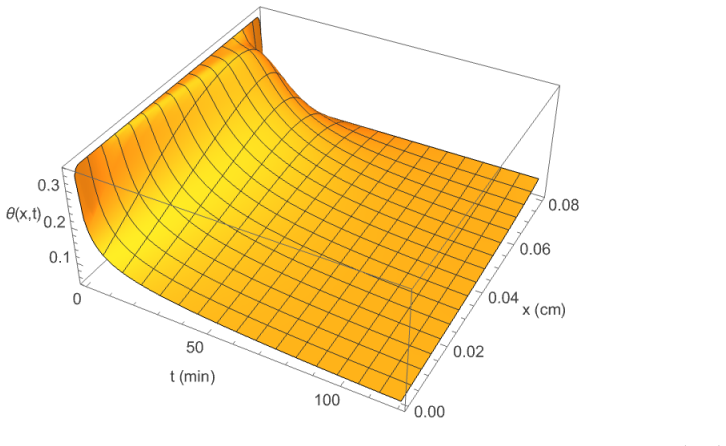
A. S. Fokas. A new transform method for evolution partial differential equations.IMA Journal of Applied Mathematics, 67(6):559–590, 2002. 11 Figure 7: Example 2: The three-dimensional visualization of the analytical solutionθ(x, t) for x∈[0,8] cm andt∈[0,120] min
work page 2002
-
[15]
A. S. Fokas and E. Kaxiras.Modern Mathematical Methods for Scientists and Engineers: a street-smart introduction. World Scientific, Singapore, 2022
work page 2022
-
[16]
R. G. Hills and A. W. Warrick. Burgers’ equation: A solution for soil water flow in a finite length.Water resources research, 29(4):1179–1184, 1993
work page 1993
-
[17]
E. Hopf. The partial differential equation.Communications on Pure and Applied Mathematics, 3:201–230, 1950
work page 1950
-
[18]
G. Hwang. Null controllability of the advection-dispersion equation with respect to the disper- sion parameter using the fokas method.International Journal of Control, 97(12):2755–2764, 2024
work page 2024
-
[19]
K. Kalimeris and L. Mindrinos. An analytical solution to the 1d drainage problem.Mathemat- ics, 13(20):3279, 2025
work page 2025
-
[20]
K. Kalimeris and L. Mindrinos. Rainfall infiltration: Direct and inverse problems on a linear evolution equation.Evolution Equations and Control Theory, 14(6):1490–1516, 2025
work page 2025
-
[21]
K. Kalimeris and T. ¨Ozsarı. An elementary proof of the lack of null controllability for the heat equation on the half line.Applied Mathematics Letters, 104:106241, 2020
work page 2020
-
[22]
K. Kalimeris, T. ¨Ozsarı, and N. Dikaios. Numerical computation of neumann controls for the heat equation on a finite interval.IEEE Transactions on Automatic Control, 69(1):161–173, 2023
work page 2023
-
[23]
D. Mantzavinos and A. S. Fokas. The unified method for the heat equation: I. non-separable boundary conditions and non-local constraints in one dimension.European Journal of Applied Mathematics, 24(6):857–886, 2013. 12
work page 2013
-
[24]
J. R. Philip. A linearization technique for the study of infiltration. In R. E. Rijtema and H. Wassink, editors,Water in the Unsaturated Zone, volume 1, pages 471–478, Paris, 1966. United Nations Educational Scentific and Cultural Organization
work page 1966
-
[25]
J. R. Philip. Recent progress in the solution of nonlinear diffusion equations.Soil Science, 117(5):257–264, 1974
work page 1974
-
[26]
L. A. Richards. Capillary conduction of liquids through porous mediums.Physics, 1(5):318– 333, 1931
work page 1931
-
[27]
A. Warrick and G. W. Parkin. Analytical solution for one-dimensional drainage: Burgers’ and simplified forms.Water resources research, 31(11):2891–2894, 1995. 13
work page 1995
discussion (0)
Sign in with ORCID, Apple, or X to comment. Anyone can read and Pith papers without signing in.