Recognition: no theorem link
A Volume of Fluid Immersed Boundary Method for Industrial Polymer Mixing
Pith reviewed 2026-05-13 05:12 UTC · model grok-4.3
The pith
A block-coupled VOF-IB solver delivers stable velocity and pressure fields for polymer mixing in partially filled screw extruders.
A machine-rendered reading of the paper's core claim, the machinery that carries it, and where it could break.
Core claim
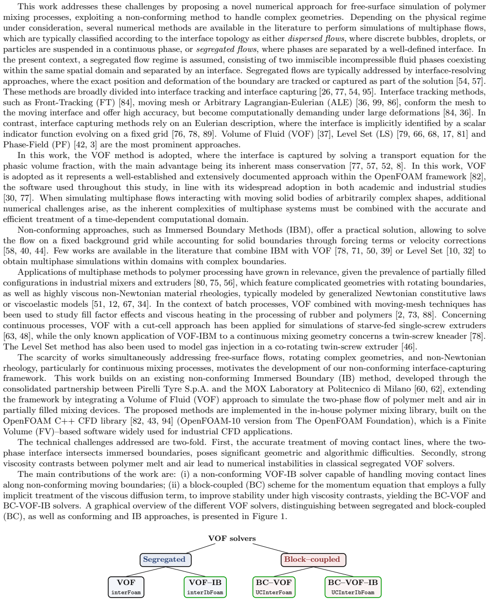
The paper presents the BC-VOF-IB solver, which integrates a volume-of-fluid interface capturing method with a non-conforming immersed boundary approach for rotating geometries. A block-coupled scheme provides fully implicit viscous diffusion treatment to overcome instabilities from strong viscosity contrasts between polymer and air. When applied to single- and twin-screw extruders, the solver delivers physically consistent velocity and pressure fields under partial filling conditions.
What carries the argument
The block-coupled VOF-IB framework, which couples volume-of-fluid free-surface tracking with immersed boundary treatment of moving parts and uses implicit viscous diffusion to stabilize high-viscosity-ratio flows.
If this is right
- Industrial geometries like single- and twin-screw extruders can now be simulated with consistent flow fields under partial fill conditions.
- Time-step stability constraints are relaxed, substantially lowering computational costs relative to segregated solvers.
- The approach provides a path toward bridging academic CFD research with the practical demands of industrial polymer processing.
- Inclusion of thermal effects would extend the framework to more realistic polymer melt behavior.
Where Pith is reading between the lines
- The same block-coupled treatment could apply to other free-surface methods or multiphase flows with large property contrasts beyond polymer-air systems.
- Validation against experimental velocity or pressure data from real extruders would provide a direct test of the physical consistency.
- The method might generalize to other rotating industrial mixers where partial filling and high viscosity ratios are common.
Load-bearing premise
The block-coupled implicit viscous treatment removes instabilities from extreme viscosity contrasts without introducing new discretization or interface errors that invalidate the velocity and pressure fields in partially filled rotating geometries.
What would settle it
If simulations of the twin-screw extruder at higher resolution produce unphysical pressure spikes or velocity discontinuities at the polymer-air interface that contradict experimental measurements, the claim of physical consistency would be falsified.
Figures


read the original abstract
This work develops advanced numerical methods for free-surface simulations of polymer mixing processes, integrating a Volume of Fluid (VOF) interface-capturing approach with a non-conforming Immersed Boundary (IB) method to model two-phase flows of highly viscous polymer melts and air within partially filled rotating mixing devices, implemented within the Finite Volume OpenFOAM library. To overcome severe numerical instabilities arising from the strong viscosity contrast between polymer melts and air, a block-coupled scheme providing fully implicit viscous diffusion treatment is integrated into the VOF-IB framework, relaxing time-step stability constraints and substantially reducing computational cost with respect to standard segregated solvers. The resulting BC-VOF-IB solver is applied to industrially relevant geometries of single- and twin-screw extruders, yielding physically consistent predictions of velocity and pressure fields under partial filling conditions. While further developments, most notably the inclusion of thermal effects, remain necessary, the proposed framework represents a meaningful step toward bridging academic CFD research and the practical demands of industrial polymer processing.
Editorial analysis
A structured set of objections, weighed in public.
Referee Report
Summary. This paper develops a Volume of Fluid (VOF) interface-capturing method combined with a non-conforming Immersed Boundary (IB) approach for two-phase simulations of highly viscous polymer melts and air in partially filled rotating mixing devices. A block-coupled implicit viscous diffusion treatment is integrated into the VOF-IB framework within OpenFOAM to address instabilities from extreme viscosity contrasts. The resulting BC-VOF-IB solver is applied to single- and twin-screw extruder geometries, with the central claim being that it yields physically consistent velocity and pressure fields under partial filling conditions.
Significance. If the stability and consistency of the fields can be confirmed, the work provides a practical numerical advance for industrial polymer processing CFD, enabling simulations of complex free-surface flows in rotating machinery that are otherwise prone to instability. The block-coupled viscous treatment is a notable technical feature for relaxing time-step constraints at high viscosity ratios, and the positioning toward industrial geometries is a strength. The explicit note on needed thermal effects is appropriately cautious.
major comments (1)
- Results section: the central claim that the solver 'yields physically consistent predictions of velocity and pressure fields' under partial filling is not supported by any quantitative validation, mesh convergence data, error norms, or comparisons to experiments/other codes. This directly affects the ability to evaluate whether the block-coupled treatment removes instabilities without introducing new interface or discretization errors in the rotating geometries.
Simulated Author's Rebuttal
We thank the referee for their constructive review and for highlighting the need for stronger support of our central claims. We address the major comment point by point below.
read point-by-point responses
-
Referee: Results section: the central claim that the solver 'yields physically consistent predictions of velocity and pressure fields' under partial filling is not supported by any quantitative validation, mesh convergence data, error norms, or comparisons to experiments/other codes. This directly affects the ability to evaluate whether the block-coupled treatment removes instabilities without introducing new interface or discretization errors in the rotating geometries.
Authors: We agree that the manuscript as submitted does not provide quantitative validation metrics such as error norms, mesh convergence studies, or direct comparisons to experiments or other codes. The results section demonstrates the solver's ability to produce stable simulations of partially filled single- and twin-screw extruders, with velocity and pressure fields that remain bounded and free of the oscillations typically seen in segregated solvers at high viscosity ratios. However, this leaves the claim of 'physical consistency' supported primarily by qualitative evidence. In the revised manuscript we will add a new subsection presenting mesh-independence results for integral quantities (e.g., screw torque and free-surface location) together with verification against limiting analytical cases for rotating viscous flows. These additions will allow a more rigorous assessment of whether the block-coupled treatment preserves accuracy while removing instabilities. revision: yes
Circularity Check
No significant circularity
full rationale
The paper constructs a numerical solver (BC-VOF-IB) by combining existing VOF and IB techniques with a block-coupled implicit viscous scheme. No derivation chain reduces a claimed prediction or result to its own inputs by construction, self-definition, or self-citation load-bearing. The central claims concern application to extruder geometries and physical consistency of fields; these are presented as outcomes of the implemented method to be assessed against external physical benchmarks rather than internal tautologies. No fitted parameters are renamed as predictions, no uniqueness theorems are imported from prior author work to force choices, and no ansatz is smuggled via citation. The work is self-contained as method development.
Axiom & Free-Parameter Ledger
Reference graph
Works this paper leans on
-
[1]
H. J. Aguerre, C. I. Pairetti, C. M. Venier, S. M´ arquez Dami´ an, and N. M. Nigro. An oscillation-free flow solver based on flux reconstruction.Journal of Computational Physics, 365:135–148, 2018
work page 2018
-
[2]
I. Ahmed and A. J. Chandy. 3D numerical investigations of the effect of fill factor on dispersive and distributive mixing of rubber under non-isothermal conditions.Polymer Engineering & Science, 59(3):535–546, 2019
work page 2019
-
[3]
D. M. Anderson, G. B. McFadden, and A. A. Wheeler. Diffuse-interface methods in fluid mechanics.Annual Review of Fluid Mechanics, 30:139–165, 1998
work page 1998
- [4]
-
[5]
E. Berberovi´ c.Numerical Investigation of Free Surface Flows including Interface Heat and Mass Transfer and Contact Line Phenomena. PhD thesis, TU Darmstadt, 2010. 25
work page 2010
- [6]
-
[7]
J. Brackbill, D. Kothe, and C. Zemach. A continuum method for modeling surface tension.Jorunal of Computational Physics, 100, 1992
work page 1992
-
[8]
A. Caboussat, V. Maronnier, M. Picasso, and J. Rappaz. Numerical simulation of three dimensional free surface flows with bubbles. InChallenges in Scientific Computing-CISC 2002: Proceedings of the Conference Challenges in Scientific Computing Berlin, October 2–5, 2002, pages 69–86. Springer, 2003
work page 2002
-
[9]
A. Caboussat, M. Picasso, and J. Rappaz. Numerical simulation of free surface incompressible liquid flows surrounded by compressible gas.Journal of Computational Physics, 203(2):626–649, 2005
work page 2005
-
[10]
A. Calderer, S. Kang, and F. Sotiropoulos. Level set immersed boundary method for coupled simulation of air/water interaction with complex floating structures.Journal of Computational Physics, 277:201–227, 2014
work page 2014
-
[11]
P. Cardiff, ˇZ. Tukovi´ c, H. Jasak, and A. Ivankovi´ c. A block-coupled finite volume methodology for linear elasticity and unstructured meshes.Computers & structures, 175:100–122, 2016
work page 2016
-
[12]
R. P. Chhabra. Non–Newtonian fluids: an introduction. InRheology of complex fluids, pages 3–34. Springer, 2010
work page 2010
-
[13]
R. Comminal, F. Pimenta, J. Spangenberg, and M. A. Alves. Experimental and numerical investigation of the die swell in 3D printing processes.Micromachines, 14(2):329, 2023
work page 2023
-
[14]
R. Courant, K. Friedrichs, and H. Lewy. ¨Uber die partiellen differenzengleichungen der mathematischen physik.Math- ematische annalen, 100(1):32–74, 1928
work page 1928
-
[15]
D. A. de Miranda, W. K. Rauber, M. Vaz Jr, M. V. C. Alves, F. H. Lafratta, A. L. Nogueira, and P. S. B. Zdanski. Analysis of numerical modeling strategies to improve the accuracy of polymer injection molding simulations.Journal of Non-Newtonian Fluid Mechanics, 315:105033, 2023
work page 2023
-
[16]
S. S. Deshpande, L. Anumolu, and M. F. Trujillo. Evaluating the performance of the two-phase flow solver interfoam. Computational Science & Discovery, 5(014016), 2012
work page 2012
-
[17]
D. A. Di Pietro, S. L. Forte, and N. Parolini. Mass preserving finite element implementations of the level set method. Applied Numerical Mathematics, 56(9):1179–1195, 2006
work page 2006
-
[18]
M. S. Dodd and A. Ferrante. A fast pressure-correction method for incompressible two-fluid flows.Journal of Compu- tational Physics, 273:416–434, 2014
work page 2014
-
[19]
T. Dong et al. Simulation of flow and mixing for highly viscous fluid in a twin screw extruder with a conveying element using parallelized smoothed particle hydrodynamics.Chemical Engineering Science, 212:115311, 2020
work page 2020
-
[20]
T. Dong, H. Liu, S. Jiang, L. Gu, Q. Xiao, Z. Yu, and X. Liu. Simulation of free surface flow with a revolving moving boundary for screw extrusion using smoothed particle hydrodynamics.CMES-Computer Modeling in Engineering & Sciences, 95(5):339–360, 2013
work page 2013
-
[21]
T. Dong and J. Wu. Simulation of non-Newtonian flows in a partially filled twin-screw extruder by smoothed particle hydrodynamics.Polymer Engineering & Science, 62(3):802–814, 2022
work page 2022
-
[22]
T. Dong, J. Wu, Y. Ruan, et al. Simulation of multiphase flow and mixing in a conveying element of a co-rotating twin-screw extruder by using SPH.International Journal of Chemical Engineering, 2023:8383763, 2023
work page 2023
-
[23]
C. Dopazo. On conditioned averages for intermittent turbulent flows.Journal of Fluid Mechanics, 81(3):433–438, 1977
work page 1977
-
[24]
K. Edwards. A designers’ guide to engineering polymer technology.Materials & Design, 19(1):57–67, 1998
work page 1998
-
[25]
M. El Ouafa, S. Vincent, and V. Le Chenadec. Monolithic solvers for incompressible two-phase flows at large density and viscosity ratios.Fluids, 6(1):23, 2021
work page 2021
-
[26]
S. Elgeti and H. Sauerland. Deforming fluid domains within the finite element method: five mesh-based tracking methods in comparison.Archives of Computational Methods in Engineering, 23(2):323–361, 2016
work page 2016
-
[27]
J. L. Favero, A. R. Secchi, N. S. M. Cardozo, and H. Jasak. Viscoelastic fluid analysis in internal and in free surface flows using the software OpenFOAM.Computers & Chemical Engineering, 34(12):1984–1993, 2010
work page 1984
-
[28]
J. H. Ferziger, M. Peric, and R. L. Street.Computational Methods for Fluid Dynamics. Springer, 4 edition, 2020
work page 2020
-
[29]
C. Galusinski and P. Vigneaux. On stability condition for bifluid flows with surface tension: Application to microfluidics. Journal of Computational Physics, 227(12):6140–6164, 2008
work page 2008
-
[30]
M. Garcia-Villalba, T. Colonius, O. Desjardins, D. Lucas, A. Mani, D. Marchisio, O. K. Matar, F. Picano, and S. Zaleski. Numerical methods for multiphase flows.International Journal of Multiphase Flow, 191:105285, 2025
work page 2025
-
[31]
A. Georgoulas, P. Koukouvinis, M. Gavaises, and M. Marengo. Numerical treatment of the interface in two-phase flows using a compressible framework in OpenFOAM: demonstration on a high velocity droplet impact case.Fluids, 6(2):78, 2021. 26
work page 2021
-
[32]
E. Guti´ errez, F. Favre, N. Balc´ azar, A. Amani, and J. Rigola. Numerical approach to study bubbles and drops evolving through complex geometries by using a level set–Moving mesh–Immersed boundary method.Chemical Engineering Journal, 349:662–682, 2018
work page 2018
- [33]
-
[34]
W. H. Herschel and R. Bulkley. Konsistenzmessungen von gummi-benzoll¨ osungen.Kolloid-Zeitschrift, 39:291–300, 1926
work page 1926
-
[35]
D. P. Hill.The computer simulation of dispersed two-phase flow. PhD thesis, Citeseer, 1998
work page 1998
-
[36]
C. Hirt, A. Amsden, and J. Cook. An arbitrary Lagrangian-Eulerian computing method for all flow speeds.Journal of Computational Physics, 14(3):227–253, 1974
work page 1974
-
[37]
C. W. Hirt and B. D. Nichols. Volume of fluid (VOF) method for the dynamics of free boundaries.Journal of Computational Physics, 39(1):201–225, 1981
work page 1981
-
[38]
P. Hold. Mixing of polymers— an overview part i.Advances in Polymer Technology, 2(2):141–151, 1982
work page 1982
- [39]
-
[40]
T. Ikeno and T. Kajishima. Finite-difference immersed boundary method consistent with wall conditions for incom- pressible turbulent flow simulations.Journal of Computational Physics, 226(2):1485–1508, Oct 2007
work page 2007
-
[41]
R. I. Issa. Solution of the implicitly discretised fluid flow equations by operator-splitting.Journal of computational physics, 62(1):40–65, 1986
work page 1986
-
[42]
D. Jacqmin. Calculation of two-phase Navier-Stokes flows using phase-field modeling.Journal of Computational Physics, 155(1):96–127, 1999
work page 1999
-
[43]
Jasak.Error Analysis and Estimation for the Finite Volume Method with Applications to Fluid Flows
H. Jasak.Error Analysis and Estimation for the Finite Volume Method with Applications to Fluid Flows. PhD thesis, Imperial College of Science, Technology and Medicine, University of London, London, United Kingdom, 1996
work page 1996
-
[44]
H. Jasak, D. Rigler, and ˇZ. Tukovi´ c. Design and implementation of immersed boundary method with discrete forcing approach for boundary conditions. In6th European Conference on Computational Fluid Dynamics, ECFD 2014, pages 5319–5332. International Center for Numerical Methods in Engineering (CIMNE), 2014
work page 2014
- [45]
-
[46]
T. M. Kousemaker, P. D. Druetta, F. Picchioni, and A. I. Vakis. Modelling supercritical CO 2 flow in a co-rotating twin screw extruder using the level-set method.Chemical Engineering Research and Design, 205:569–577, 2024
work page 2024
-
[47]
C.-Y. Ku. A novel method for solving ill-conditioned systems of linear equations with extreme physical property contrasts.CMES, 96(6):409–434, 2013
work page 2013
-
[48]
M. R. Larsen, E. T. Holmen Olofsson, J. H. Hattel, and J. Spangenberg. Numerical investigation of continuous mixing of highly viscous, non-Newtonian polymer suspensions by a starved-fed single-screw extruder. InAIP Conference Proceedings, volume 3158, page 070004. AIP Publishing, 2024
work page 2024
-
[49]
M. R. Larsen, T. Ottsen, E. T. Holmen Olofsson, and J. Spangenberg. Numerical modeling of the mixing of highly viscous polymer suspensions in partially filled sigma blade mixers.Polymers, 15(8):1938, 2023
work page 1938
- [50]
-
[51]
C. W. Macosko.Rheology: Principles, Measurements and Applications. Wiley, 1994
work page 1994
-
[52]
V. Maronnier, M. Picasso, and J. Rappaz. Numerical simulation of free surface flows.Journal of Computational Physics, 155(2):439–455, 1999
work page 1999
-
[53]
J. A. D. Marquez, Y. Quan, X. Zhu, H.-J. Sue, and Q. Wang. Predicting the processability of polymers in a twin-screw extruder: CFD simulation and experimental validation.Industrial & Engineering Chemistry Research, 63(22):9823–9832, 2024
work page 2024
-
[54]
Marschall.Towards the numerical simulation of multi-scale two-phase flows
H. Marschall.Towards the numerical simulation of multi-scale two-phase flows. PhD thesis, Technische Universit¨ at M¨ unchen, 2011
work page 2011
-
[55]
T. Matzerath and C. Bonten. Automated optimization of mixing elements for single-screw extrusion using CFD simu- lations.Polymers, 17(4):438, 2025
work page 2025
-
[56]
Middleman.Fundamentals of Polymer Processing
S. Middleman.Fundamentals of Polymer Processing. McGraw-Hill, New York, 1977
work page 1977
-
[57]
S. Mirjalili, S. Jain, and M. Dodd. Interface-capturing methods for two-phase flows: An overview and recent develop- ments.Center for Turbulence Research - Annual research brief, pages 117–135, 12 2017
work page 2017
-
[58]
R. Mittal and G. Iaccarino. Immersed boundary methods.Annual Review of Fluid Mechanics, 37:239–261, 2005. 27
work page 2005
-
[59]
F. Moukalled, L. Mangani, and M. Darwish.The Finite Volume Method in Computational Fluid Dynamics: An Advanced Introduction with OpenFOAM® and Matlab, volume 113 ofFluid Mechanics and Its Applications. Springer International Publishing, Cham, Switzerland, 2016
work page 2016
-
[60]
Negrini.Non-conforming methods for the simulation of industrial polymer mixing processes
G. Negrini.Non-conforming methods for the simulation of industrial polymer mixing processes. PhD thesis, Politecnico di Milano, 2023
work page 2023
-
[61]
G. Negrini, N. Parolini, and M. Verani. On the convergence of the Rhie–Chow stabilized box method for the Stokes problem.International Journal for Numerical Methods in Fluids, 96(8):1489–1516, 2024
work page 2024
-
[62]
G. Negrini, N. Parolini, and M. Verani. An immersed boundary method for polymeric continuous mixing. InEmerging Technologies in Computational Sciences for Industry, Sustainability and Innovation, pages 163–178. Springer Nature Switzerland, 2025
work page 2025
-
[63]
E. H. Olofsson, M. Roland, J. Spangenberg, N. H. Jokil, and J. H. Hattel. A CFD model with free surface tracking: predicting fill level and residence time in a starve-fed single-screw extruder.The International Journal of Advanced Manufacturing Technology, 126(7):3579–3591, 2023
work page 2023
-
[64]
E. Olsson and G. Kreiss. A conservative level set method for two phase flow.Journal of computational physics, 210(1):225–246, 2005
work page 2005
- [65]
-
[66]
S. Osher and J. A. Sethian. Fronts propagating with curvature-dependent speed: algorithms based on Hamilton–Jacobi formulations.Journal of Computational Physics, 79(1):12–49, 1988
work page 1988
-
[67]
W. Ostwald. Concerning the function rate of the viscosity of dispersion systems.Kolloid-Zeitschrift, 36:99–117, 1925
work page 1925
-
[68]
N. Parolini and E. Burman. A finite element level set method for viscous free-surface flows. InApplied and industrial mathematics in Italy, pages 416–427. World Scientific, 2005
work page 2005
-
[69]
S. V. Patankar.Numerical Heat Transfer and Fluid Flow. Series in Computational Methods in Mechanics and Thermal Sciences. Hemisphere Publishing Corporation, 1980
work page 1980
-
[70]
S. V. Patankar and D. B. Spalding. A calculation procedure for heat, mass and momentum transfer in three-dimensional parabolic flows.International Journal of Heat and Mass Transfer, 15(10):1787–1806, 1972
work page 1972
-
[71]
H. V. Patel et al. A coupled Volume of Fluid and Immersed Boundary Method for simulating 3D multiphase flows with contact line dynamics in complex geometries.Chemical Engineering Science, 166:28–41, 2017
work page 2017
-
[72]
F. Pimenta and M. A. Alves. Stabilization of an open-source finite-volume solver for viscoelastic fluid flows.Journal of Non-Newtonian Fluid Mechanics, 239:85–104, 2017
work page 2017
-
[73]
H. Poudyal, I. Ahmed, and A. J. Chandy. Three-dimensional, non-isothermal simulations of the effect of speed ratio in partially-filled rubber mixing.International Polymer Processing, 34(2):219–230, 2019
work page 2019
-
[74]
S. Rajendran, R. M. Manglik, and M. A. Jog. New property averaging scheme for volume of fluid method for two-phase flows with large viscosity ratios.Journal of Fluids Engineering, 144(6):061101, 2022
work page 2022
-
[75]
C. Rauwendaal.Polymer extrusion. Carl Hanser Verlag GmbH Co KG, 2014
work page 2014
-
[76]
Rusche.Computational Fluid Dynamics of Dispersed Two-Phase Flows at High Phase Fractions
H. Rusche.Computational Fluid Dynamics of Dispersed Two-Phase Flows at High Phase Fractions. PhD thesis, Imperial College of Science, Technology and Medicine, 01 2002
work page 2002
-
[77]
R. Scardovelli and S. Zaleski. Direct numerical simulation of free-surface and interfacial flow.Annu. Rev. Fluid Mech., 31, 01 1999
work page 1999
- [78]
-
[79]
M. Sussman, P. Smereka, and S. Osher. A level set approach for computing solutions to incompressible two-phase flow. Journal of Computational Physics, 114(1):146–159, 1994
work page 1994
-
[80]
Z. Tadmor and C. G. Gogos.Principles of polymer processing. John Wiley & Sons, 2013
work page 2013
discussion (0)
Sign in with ORCID, Apple, or X to comment. Anyone can read and Pith papers without signing in.