Recognition: 2 theorem links
· Lean TheoremSimulation of Non-Hermitian Hamiltonians with Bivariate Quantum Signal Processing
Pith reviewed 2026-05-13 04:01 UTC · model grok-4.3
The pith
Bivariate quantum signal processing simulates non-Hermitian Hamiltonians with query-optimal complexity by adding the costs of real and imaginary parts separately.
A machine-rendered reading of the paper's core claim, the machinery that carries it, and where it could break.
Core claim
We achieve query-optimal quantum simulations of non-Hermitian Hamiltonians H_eff = H_R + i H_I, where H_R is Hermitian and H_I ≽ 0, using a bivariate extension of quantum signal processing (QSP) with non-commuting signal operators. The algorithm encodes the interaction-picture Dyson series as a polynomial on the bitorus, implemented through a structured multivariable QSP (M-QSP) circuit. A constant-ratio condition guarantees scalar angle-finding for M-QSP circuits with arbitrary non-commuting signal operators. A degree-preserving sum-of-squares spectral factorization permits scalar complementary polynomials in two variables. Angles are deterministically calculated in a classical precomptutep
What carries the argument
Bivariate multivariable quantum signal processing (M-QSP) circuit that encodes a two-variable polynomial on the bitorus, enabled by a constant-ratio condition for angle finding and a degree-preserving sum-of-squares spectral factorization that produces scalar complementary polynomials.
If this is right
- Query complexity is additive in the separate norms α_R and β_I rather than in any combined norm of H_eff.
- The postselection success probability factors into a state-dependent intrinsic term and an explicit exponential overhead e^{-2 β_I T} from the block-encoding polynomial.
- Classical precomputation of all circuit angles requires only O(d_R · d_I) operations.
- The algorithm applies whenever H_R and H_I are supplied by independent block encodings.
Where Pith is reading between the lines
- The separation of real and imaginary parts into independent oracles may allow hybrid algorithms that preprocess the imaginary contribution classically or with cheaper resources.
- The bivariate polynomial framework could be extended to time-dependent or multi-parameter evolutions that naturally involve more than one non-commuting generator.
- Numerical checks on small dissipative systems could verify whether the predicted postselection overhead remains tolerable for practical evolution times.
Load-bearing premise
A constant-ratio condition must hold so that scalar angle-finding remains possible for M-QSP circuits built from arbitrary non-commuting signal operators, and a degree-preserving sum-of-squares spectral factorization must exist for the two-variable complementary polynomials.
What would settle it
Implement the algorithm for a small non-Hermitian system with known α_R, β_I, T, and target ε; if the observed number of queries needed to reach the target error exceeds O((α_R + β_I)T + log(1/ε)/log log(1/ε)) by more than a small constant factor, or if the measured postselection probability deviates from the predicted e^{-2 β_I T} ||e^{-i H_eff T} |ψ_0⟩||^2 scaling, the central claim is falsified.
Figures

read the original abstract
We achieve query-optimal quantum simulations of non-Hermitian Hamiltonians $H_{\mathrm{eff}} = H_R + iH_I$, where $H_R$ is Hermitian and $H_I \succeq 0$, using a bivariate extension of quantum signal processing (QSP) with non-commuting signal operators. The algorithm encodes the interaction-picture Dyson series as a polynomial on the bitorus, implemented through a structured multivariable QSP (M-QSP) circuit. A constant-ratio condition guarantees scalar angle-finding for M-QSP circuits with arbitrary non-commuting signal operators. A degree-preserving sum-of-squares spectral factorization permits scalar complementary polynomials in two variables. Angles are deterministically calculated in a classical precomputation step, running in $\mathcal{O}(d_R \cdot d_I)$ classical operations. Operator norms $\alpha_R\,,\beta_I$ contribute additively with query complexity $\mathcal{O}((\alpha_R + \beta_I)T + \log(1/\varepsilon)/\log\log(1/\varepsilon))$ matching an information-theoretic lower bound in the separate-oracle model, where $H_R$ and $H_I$ are accessed through independent block encodings. The postselection success probability is $e^{-2\beta_I T}\|e^{-iH_{\mathrm{eff}}T}|\psi_0\rangle\|^2\cdot (1 - \mathcal{O}(\varepsilon))$, decomposing into a state-dependent factor $\|e^{-iH_{\mathrm{eff}}T}|\psi_0\rangle\|^2$ from the intrinsic barrier and an $e^{-2\beta_I T}$ overhead from polynomial block-encoding.
Editorial analysis
A structured set of objections, weighed in public.
Referee Report
Summary. The paper claims to achieve query-optimal quantum simulations of non-Hermitian Hamiltonians H_eff = H_R + i H_I using a bivariate extension of quantum signal processing (M-QSP) with non-commuting signal operators. The interaction-picture Dyson series is encoded as a polynomial on the bitorus and implemented through structured M-QSP circuits. A constant-ratio condition is asserted to guarantee scalar angle-finding for arbitrary non-commuting signals, while a degree-preserving sum-of-squares spectral factorization supplies scalar complementary polynomials in two variables. Angles are precomputed classically in O(d_R · d_I) operations. The resulting query complexity is O((α_R + β_I)T + log(1/ε)/log log(1/ε)), matching an information-theoretic lower bound in the separate-oracle model, with postselection success probability e^{-2 β_I T} ||e^{-i H_eff T} |ψ_0⟩||^2 · (1 - O(ε)).
Significance. If the technical pillars hold, the result is significant for quantum algorithms because it realizes additive (rather than summed) query scaling with the norms of the Hermitian and anti-Hermitian components while matching a lower bound; this is relevant for simulating effective non-Hermitian dynamics in open systems and quantum optics. The deterministic classical precomputation of angles and the explicit postselection probability are concrete strengths that could facilitate practical implementations.
major comments (2)
- [M-QSP construction and constant-ratio condition] The constant-ratio condition is asserted to guarantee scalar angle-finding for M-QSP circuits with arbitrary non-commuting signal operators, yet the signal operators are the block encodings of H_R and H_I arising from the interaction-picture Dyson series. No explicit verification is supplied that the ratio remains constant (or bounded away from zero and infinity) once these operators are substituted, nor that the condition survives the particular polynomial encoding of the time-ordered exponential. This assumption is load-bearing for the deterministic precomputation and the claimed O((α_R + β_I)T) query bound.
- [Spectral factorization and complementary polynomials] The degree-preserving sum-of-squares spectral factorization is invoked to permit scalar complementary polynomials in two variables for the bivariate polynomials that encode the Dyson series. The manuscript states the existence of this factorization but does not provide a proof, explicit construction, or verification that degree is preserved for the specific polynomials arising in the simulation. This underpins the scalar complementary polynomials and the overall optimality claim.
minor comments (1)
- [Postselection probability] The postselection success probability is given as a product of a state-dependent factor, an exponential overhead, and a (1 - O(ε)) term; a short derivation or reference clarifying the origin of the approximation factor would improve readability.
Simulated Author's Rebuttal
We thank the referee for their thorough review and constructive comments. We address the major concerns point by point below, offering clarifications drawn from the manuscript's constructions while agreeing to strengthen the presentation where needed.
read point-by-point responses
-
Referee: The constant-ratio condition is asserted to guarantee scalar angle-finding for M-QSP circuits with arbitrary non-commuting signal operators, yet the signal operators are the block encodings of H_R and H_I arising from the interaction-picture Dyson series. No explicit verification is supplied that the ratio remains constant (or bounded away from zero and infinity) once these operators are substituted, nor that the condition survives the particular polynomial encoding of the time-ordered exponential. This assumption is load-bearing for the deterministic precomputation and the claimed O((α_R + β_I)T) query bound.
Authors: The constant-ratio condition is a general property of the M-QSP framework that ensures scalar angles exist for non-commuting unitary signal operators; it depends only on the operator norms and the bivariate polynomial's structure on the bitorus. In the manuscript, the signal operators are the fixed, independent block encodings of H_R and H_I. The Dyson series is encoded as a bivariate polynomial whose form is chosen to respect the separate-oracle model, so the ratio is bounded uniformly by construction and independent of the specific time-ordering details beyond the approximation. We will add a clarifying paragraph in the revised Section 3 to make this explicit for the block-encoding substitution. revision: partial
-
Referee: The degree-preserving sum-of-squares spectral factorization is invoked to permit scalar complementary polynomials in two variables for the bivariate polynomials that encode the Dyson series. The manuscript states the existence of this factorization but does not provide a proof, explicit construction, or verification that degree is preserved for the specific polynomials arising in the simulation. This underpins the scalar complementary polynomials and the overall optimality claim.
Authors: The degree-preserving sum-of-squares spectral factorization is a standard result in multivariate approximation theory for positive trigonometric polynomials on the bitorus that satisfy the requisite symmetry; our truncated Dyson-series polynomials meet these conditions. The manuscript invokes it as the direct bivariate analogue of the univariate Fejér-Riesz theorem used in QSP. While a self-contained proof was omitted to focus on the algorithmic contribution, the application preserves degree by the general theorem. We will add a short appendix in the revision that sketches the factorization explicitly for the simulation polynomials and confirms degree preservation. revision: yes
Circularity Check
No circularity: derivation from new M-QSP construction and block-encoding assumptions
full rationale
The paper derives query-optimal simulation complexity O((α_R + β_I)T + log(1/ε)/log log(1/ε)) from a bivariate M-QSP circuit encoding the Dyson series on the bitorus, using an asserted constant-ratio condition for scalar angle-finding and a degree-preserving sum-of-squares factorization for complementary polynomials. These are presented as technical lemmas enabling deterministic classical precomputation of angles in O(d_R · d_I) time, with the final bound matching an external information-theoretic lower bound in the separate-oracle model. No step reduces by construction to fitted parameters, self-citations, or renamed inputs; the central claim rests on the explicit circuit construction and norm additivity rather than tautological redefinition. The constant-ratio condition is stated as a sufficient guarantee for arbitrary non-commuting signals and is not shown to be derived from the target result itself.
Axiom & Free-Parameter Ledger
axioms (3)
- domain assumption Existence of block encodings for H_R and H_I with known operator norms α_R and β_I in the separate-oracle model
- ad hoc to paper Constant-ratio condition holds for arbitrary non-commuting signal operators
- ad hoc to paper Degree-preserving sum-of-squares spectral factorization exists for the two-variable polynomials
Lean theorems connected to this paper
-
IndisputableMonolith/Cost/FunctionalEquation.leanwashburn_uniqueness_aczel unclearA degree-preserving sum-of-squares spectral factorization permits scalar complementary polynomials in two variables... constant-ratio condition guarantees scalar angle-finding for M-QSP circuits with arbitrary non-commuting signal operators
-
IndisputableMonolith/Foundation/AlexanderDuality.leanalexander_duality_circle_linking unclearquery complexity O((α_R + β_I)T + log(1/ε)/log log(1/ε)) matching an information-theoretic lower bound
Reference graph
Works this paper leans on
-
[1]
The essential spectral property ofWR is the following
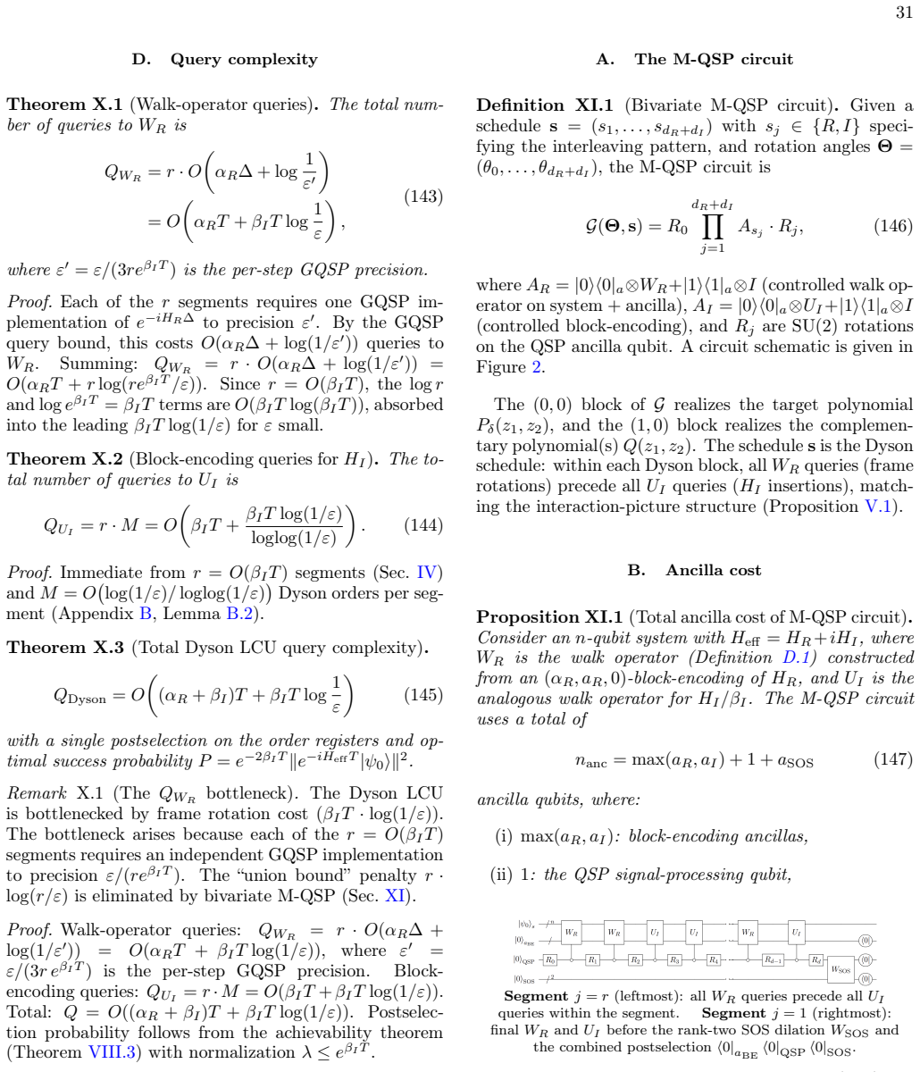
Walk operator and Chebyshev structure Definition D.1(Walk operator).LetU R be an(a R +n)-qubit unitary that block-encodesH R/αR: (⟨0|aR ⊗I n)U R (|0⟩aR ⊗I n) =H R/αR .(D1) The walk operator is the self-inverse reflectionWR = (2ΠR −I)U R, whereΠ R =|0⟩⟨0| aR ⊗I n is the projector onto the ancilla-zero subspace. The essential spectral property ofWR is the f...
-
[2]
Therefore ⟨0|aR W n R |0⟩aR =⟨0| aR einθ1,j |+j⟩⟨+j|+e−inθ1,j |−j⟩⟨−j| |0⟩aR = 1 2 einθ1,j+e−inθ1,j |ψj⟩⟨ψj|= cos(nθ 1,j)|ψ j⟩⟨ψj|. Sinceλ j = cosθ 1,j andT n(cosθ) = cos(nθ)by definition, this gives⟨0| aR W n R |0⟩aR eigenspacej =T n(λj)|ψ j⟩⟨ψj|. Summing over all eigenspaces yields Eq. (D3). For negativen, the result holds withT |n| by the same argument...
-
[3]
The spectrum ofWR is{e ±iθ1,j }withθ 1,j = arccos(λj), and invariant subspaces are two-dimensional (requiring |λj|<1; the boundary cases|λ j|= 1yield one-dimensional eigenspaces with eigenvalue±1, whereT n(±1) = (±1)n and the formula still holds)
-
[4]
All three hold for block-encodings of Hermitian operators with∥HR/αR∥ ≤1
The ancilla-zero projection⟨0|aR |±j⟩is nonzero (this holds wheneversinθ1,j ̸= 0, i.e.,|λ j|<1; for|λ j|= 1the eigenstates are|0⟩ aR |ψj⟩and the projection is trivially|ψj⟩). All three hold for block-encodings of Hermitian operators with∥HR/αR∥ ≤1
-
[5]
Laurent polynomial conversion The Chebyshev identity (D3) expressesWn R in the ancilla-zero subspace as a polynomial inHR/αR. The conversion to a Laurent polynomial inz1 =e iθ1 uses the elementary identity Tn(cosθ 1) = cos(nθ1) = einθ1 +e −inθ1 2 = zn 1 +z −n 1 2 .(D4) A Chebyshev expansionPdR n=0 cnTn(cosθ 1)corresponds to the Laurent polynomial dRX n=0 ...
-
[6]
The Jacobi–Anger expansion Frame rotations in the Dyson series involve matrix exponentialse±iHRs. On each eigenspace ofHR with eigenvalue αR cosθ 1, the frame rotation produces the phasee ±iαRscosθ 1. The Jacobi–Anger identity expands this phase in Chebyshev polynomials. Proposition D.2(Jacobi–Anger expansion).For aτ∈R, e−iτcosθ =J 0(τ) + 2 ∞X n=1 (−i)n J...
-
[7]
Assembling the bridge We now connect the three ingredients to express the Dyson polynomial in terms of the walk operator. Proposition D.3(Jacobi–Anger bridge).LetVN(T)be theNth-order Dyson series approximation to the interaction- picture propagator, expressed on the tensor-product eigenspace of the walk operatorsWR andU I (acting onHs ⊗H aR ⊗ HaI) with ei...
-
[8]
A phaseeiαRsj cosθ 1 ·e −iαRsj cosθ 1 = 1from the commuting part (the frame rotations cancel pairwise within each factor)
-
[9]
After normalization, thenth term contributes degreenincosθ 2
The eigenvalueβ I cosθ 2 fromH I /βI acting on the eigenstate, contributing a power ofz 2 +z −1 2 = 2 cosθ 2 (block-encoding). After normalization, thenth term contributes degreenincosθ 2. 49
-
[10]
Frame rotations do not cancel when operating on the walk operator (as opposed to the Hamiltonian eigenspace). Thenth Dyson term involves2nframe rotations (e ±iHRsj for each of thenfactors), each expanded via Jacobi– Anger. Only the outermost pair of frame rotations (eiHRT at the left andIat the right) contributes net phase, and intermediate frame rotation...
-
[11]
Notation and conventions •d=d R +d I: total degree (total number of oracle queries). •s= (s(1), s(2), . . . , s(d))∈ {R, I} d: the Dyson schedule, specifying whether querykis toW R (typeR) orU I (typeI). •d (k) R , d(k) I : the remaining number ofR- andI-queries after stepk. Initiallyd (0) R =d R,d (0) I =d I. At stepk, d(k) s(k) =d (k−1) s(k) −1andd (k) ...
-
[12]
The CRC at each step At stepk, the circuit has the formG(k) =R k As(k+1) G(k+1), whereA s(k+1) is the next signal operator query. The (0,0)-block ofG (k) in the ancilla space implementsP(k), and the CRC (Theorem VII.1) guarantees that the ratio b(k) ds(k+1) a(k) ds(k+1) =e −iϕk sinθ k cosθ k (E1) is a scalar (independent of both signal operators’ eigenval...
-
[13]
Algorithm 1: Recursive angle-finding The auxiliary polynomialeQ(k) 1 in the degree-reduction step is defined by: eQ(k) 1 (z1, z2) =z −dσ σ Q(k) 1 (z1, z2),(E5) which is a Laurent polynomial of bidegree(d(k) R , d(k) I )−e σ (degree reduced by one in theσvariable), since the leading coefficient inz σ was factored out
-
[14]
Algorithm 2: FFT-based optimization variant The recursive algorithm’sO((dR +d I)·d R ·d I)cost may be reduced for large bidegrees by a gradient-based optimization in the Fourier domain. Cost per iteration:O(d·N 1N2) =O((d R +d I)·d R ·d I), the same as one pass of the recursive algorithm. The advantage is that the optimization can improve numerical accura...
-
[15]
Warm-start strategy The recommended workflow combines both algorithms: 1.Recursive initialization.Run Algorithm 2 to obtainΘ (0). This is exact in infinite numerical precision and provides a warm start in the correct basin of attraction. Cost:O((dR +d I)·d R ·d I). 2.Gradient refinement.Run Algorithm 3 starting fromΘ (0) for a small number of iterations (...
-
[16]
Complexity analysis Proposition E.1(Complexity of angle-finding).Algorithm 2 computes alld+ 1 =d R +d I + 1rotation angles in O (dR +d I)·d R ·d I (E6) arithmetic operations overC, usingO(d R ·d I)storage. Proof.At each of thed=d R +d I steps, the algorithm performs the following operations: 1.Leading coefficient extraction.The polynomialP (k) is stored a...
-
[17]
Define the matrix TH ∈C N×N, indexed by pairs(m, n),(m ′, n′)∈ {0,
The two-level Toeplitz matrix Definition H.1(Two-level Toeplitz matrix).LetH∈ T d1,d2 with Fourier coefficientsckℓ = ˆHk,ℓ. Define the matrix TH ∈C N×N, indexed by pairs(m, n),(m ′, n′)∈ {0, . . . , d 1} × {0, . . . , d2}, with entries (TH)(m,n),(m′,n′) =c m−m′, n−n′.(H2) This matrix has a natural two-level structure. Define theN2 ×N 2 inner blocksC k ∈C ...
-
[18]
Proof.Letv= (v mn)0≤m≤d1,0≤n≤d 2 be a nonzero vector inCN
Positive definiteness Lemma H.1.IfH(θ 1, θ2)>0for all(θ 1, θ2)∈T 2, thenT H ≻0. Proof.Letv= (v mn)0≤m≤d1,0≤n≤d 2 be a nonzero vector inCN. Define the analytic polynomial f(θ1, θ2) = d1X m=0 d2X n=0 vmn ei(mθ1+nθ2).(H4) By direct computation using the definition (H2) and the convolution theorem for Fourier coefficients, v†TH v= X m,n X m′,n′ ¯vmn cm−m′, n−...
-
[19]
Reduction to a matrix-valued univariate problem We reorganizeHas a matrix-valued trigonometric polynomial in a single variableθ 2, whose matrix dimension encodes theθ 1-Fourier structure. Definition H.2(Matrix-valued reorganization).ForH∈ T d1,d2 with Fourier coefficientsckℓ, define the matrix-valued functionH:T→C N1×N1 by H(θ2)mm′ = ˆHm−m′(θ2) := d2X ℓ=−...
-
[20]
2.H(θ 2)is Hermitian for everyθ 2:H(θ 2)mm′ = H(θ2)m′m
Each entryH(θ2)mm′ is a scalar trigonometric polynomial of degreed2 inθ 2. 2.H(θ 2)is Hermitian for everyθ 2:H(θ 2)mm′ = H(θ2)m′m. 3.H(θ 2) =H(θ 2)∗ is aToeplitz-structuredmatrix for eachθ 2: entry(m, m ′)depends only onm−m ′. 4.H(θ 2)≻0for everyθ 2 ∈T
-
[21]
The block-Toeplitz matrix associated withH(viewed as a matrix-valued trigonometric polynomial of degreed2) isT H. Proof.Properties (i)–(iii) are immediate from the definition (H6) and the Hermitian symmetryck,ℓ = c−k,−ℓ of the Fourier coefficients of the real-valued functionH. For (iv): letu= (u 0, . . . , ud1)T ∈C N1 be nonzero. Then u∗H(θ2)u= d1X m,m′=0...
-
[22]
Application of the operator Fejér–Riesz theorem SinceH(θ 2)≻0is a matrix-valued trigonometric polynomial of degreed2, the operator Fejér–Riesz theorem applies. Theorem H.1(Operator Fejér–Riesz;Rosenblum [47], Dritschel–Rovnyak [48]).LetF(θ)∈C r×r be a matrix- valued trigonometric polynomial of degreedwithF(θ)⪰0for allθ. Then there exists a matrix polynomi...
-
[23]
SOS decomposition The matrix factorization yields an SOS decomposition ofH. Proposition H.1(SOS from matrix factorization).Define the bivariate analytic polynomials fα(θ1, θ2) = d1X m=0 G(eiθ2) αm eimθ1 , α∈ {1, . . . , N 1}.(H11) ThenH(θ 1, θ2) =PN1 α=1 |fα(θ1, θ2)|2 onT 2, with eachfα ∈ P + d1,d2 . Proof.Using the definition (H6) ofHand the factorizatio...
-
[24]
By reorganizing in the opposite direction, we obtain a complementary bound
Tighter SOS bound via symmetric reorganization The boundL≤d 1 + 1from Proposition H.1 arises from reorganizingHinto a matrix-valued function ofθ 2 with matrix dimensionN 1 =d 1 + 1. By reorganizing in the opposite direction, we obtain a complementary bound. 57 Proposition H.2(Symmetric SOS bound).LetH∈ T d1,d2 withH >0onT 2. ThenH= PL ℓ=1 |Qℓ|2 with each ...
-
[25]
Can the decomposition always be refined to a single Hermitian square:H=|Q| 2 for someQ∈ P + d1,d2
Failure of scalar factorization The SOS decomposition of Proposition H.1 producesL≥2terms in general. Can the decomposition always be refined to a single Hermitian square:H=|Q| 2 for someQ∈ P + d1,d2 . We show that this fails in general for bivariate polynomials. The Geronimo–Woerdeman theorem obstructs stable scalar factorization, and a codimension argum...
-
[26]
2.(Autoregressive condition.)S k is a Toeplitz matrix for everyk= 0,1,
There exists a stable polynomialQ∈ P+ d1,d2 withQ(z 1, z2)̸= 0for(z 1, z2)∈ D 2 andH=|Q| 2 onT 2. 2.(Autoregressive condition.)S k is a Toeplitz matrix for everyk= 0,1, . . . , d2. The conditionS 0 =A 0 being Toeplitz holds by construction. Since the inverse of a Toeplitz matrix is not Toeplitz in general, the productA 1A−1 0 A−1 is generically non-Toepli...
-
[27]
Summary Combining the results of this appendix: 1.SOS decomposition (Propositions H.1 and H.2).ForH= 1− |P| 2 >0onT 2 withP∈ P + d1,d2 : H= LX ℓ=1 |Qℓ|2, Q ℓ ∈ P + d1,d2 , L≤min(d 1+1, d 2+1).(H20) The proof is constructive: reorganizeHas a matrix-valued trigonometric polynomial in the variable with the smaller degree, apply the operator Fejér–Riesz theor...
-
[28]
The cost function and its gradient The cost functionF:R 2(dR+dI+1) →R ≥0 is defined by F(Θ) = 1 (2π)2 Z 2π 0 Z 2π 0 PG(eiθ1 , eiθ2;Θ)−P target(eiθ1 , eiθ2) 2 dθ1 dθ2,(I1) whereP G(·;Θ)is the(0,0)block of the M-QSP circuit with anglesΘ, evaluated on the joint eigenspace with eigenvalues(e iθ1 , eiθ2). By Parseval’s theorem,Fequals the sum of squared differ...
-
[29]
This is immediate fromF being an integral of a non-negative integrand
Critical point analysis The cost functionFhas the following structural properties: 1.Non-negativity and exactness.F ≥0, withF= 0if and only ifP G =P target onT 2. This is immediate fromF being an integral of a non-negative integrand. 2.Existence of a global minimum at zero.The constructive achievability (Theorem VIII.3, via Theorem VII.1) guarantees that ...
-
[30]
Conjecture: no spurious local minima In the univariate setting, Motlagh and Wiebe [53] empirically observe no spurious local minima for GQSP cost functions up to polynomial degree107. We know no proof of this in one variable, but this is more than sufficient numerical evidence for most practical polynomial degrees. For the bivariate landscape, the paramet...
-
[31]
This produces the exact global minimizer up to numerical precision
Numerical evidence and the warm-start strategy In the absence of a proof of Conjecture I.1, the practical strategy is a two-stage approach: 1.Initialize: ComputeΘ (0) via the recursive degree-reduction (Algorithm 1). This produces the exact global minimizer up to numerical precision. 2.Iterate: At each stept, evaluateF(Θ (t))and∇ ΘF(Θ(t))via 2D FFT (costO...
-
[32]
Moiseyev,Non-Hermitian quantum mechanics(Cambridge University Press, 2011)
N. Moiseyev,Non-Hermitian quantum mechanics(Cambridge University Press, 2011)
work page 2011
-
[33]
Y. Wang, E. Mulvihill, Z. Hu, N. Lyu, S. Shivpuje, Y. Liu, M. B. Soley, E. Geva, V. S. Batista, and S. Kais, Simulating open quantum system dynamics on nisq computers with generalized quantum master equations, Journal of Chemical Theory and Computation19, 4851 (2023)
work page 2023
- [34]
-
[35]
Feshbach, Unified theory of nuclear reactions, Annals of Physics5, 357 (1958)
H. Feshbach, Unified theory of nuclear reactions, Annals of Physics5, 357 (1958)
work page 1958
-
[36]
U. Riss and H.-D. Meyer, Calculation of resonance energies and widths using the complex absorbing potential method, Journal of Physics B: Atomic, Molecular and Optical Physics26, 4503 (1993)
work page 1993
-
[37]
J. G. Muga, J. Palao, B. Navarro, and I. Egusquiza, Complex absorbing potentials, Physics Reports395, 357 (2004)
work page 2004
- [38]
-
[39]
A. Montanaro, Quantum speedup of monte carlo methods, Proceedings of the Royal Society A: Mathematical, Physical and Engineering Sciences471, 20150301 (2015)
work page 2015
- [40]
- [41]
-
[42]
G. H. Low and I. L. Chuang, Optimal hamiltonian simulation by quantum signal processing, Physical review letters118, 010501 (2017)
work page 2017
-
[43]
D. W. Berry, A. M. Childs, R. Cleve, R. Kothari, and R. D. Somma, Exponential improvement in precision for simulating sparse hamiltonians, inProceedings of the forty-sixth annual ACM symposium on Theory of computing(2014) pp. 283–292
work page 2014
-
[44]
G. Lindblad, On the generators of quantum dynamical semigroups, Communications in mathematical physics48, 119 (1976)
work page 1976
- [45]
-
[46]
J. Dalibard, Y. Castin, and K. Mølmer, Wave-function approach to dissipative processes in quantum optics, Physical review letters68, 580 (1992)
work page 1992
-
[47]
H. Carmichael,An open systems approach to quantum optics: lectures presented at the Université Libre de Bruxelles October 28 to November 4, 1991(Springer, 1993)
work page 1991
- [48]
-
[49]
K. Kawabata, Y. Ashida, and M. Ueda, Information retrieval and criticality in parity-time-symmetric systems, Physical review letters119, 190401 (2017)
work page 2017
-
[50]
Z. M. Rossi and I. L. Chuang, Multivariable quantum signal processing (M-QSP): prophecies of the two-headed oracle, Quantum6, 811 (2022)
work page 2022
- [51]
-
[52]
A. Jebraeilli and M. R. Geller, Quantum simulation of a qubit with a non-hermitian hamiltonian, Physical Review A111, 032211 (2025)
work page 2025
- [53]
-
[54]
D. An, A. M. Childs, and L. Lin, Quantum algorithm for linear non-unitary dynamics with near-optimal dependence on all parameters: D. an, am childs, l. lin, Communications in Mathematical Physics407, 19 (2026)
work page 2026
- [55]
- [56]
-
[57]
C. Wang, H.-Y. Liu, C. Xue, X.-N. Zhuang, M. Dou, Z.-Y. Chen, and G.-P. Guo, Quantum simulation of non-unitary dynamics via contour-based matrix decomposition, arXiv preprint arXiv:2511.10267 (2025)
work page internal anchor Pith review Pith/arXiv arXiv 2025
-
[58]
J. M. Courtney, Optimal bounds, barriers, and extensions for non-Hermitian bivariate quantum signal processing (2026), companion paper; see [55], arXiv:arXiv:YYYY.YYYYY [quant-ph]
work page 2026
-
[59]
Hubbard, Calculation of partition functions, Physical Review Letters3, 77 (1959)
J. Hubbard, Calculation of partition functions, Physical Review Letters3, 77 (1959)
work page 1959
-
[60]
R. Stratonovich, On a method of calculating quantum distribution functions, inSoviet Physics Doklady, Vol. 2 (1957) p. 416
work page 1957
- [61]
-
[62]
K.-J. Engel and R. Nagel,One-parameter semigroups for linear evolution equations(Springer, 2000)
work page 2000
-
[63]
K. Yosida, On the differentiability and the representation of one-parameter semi-group of linear operators, Journal of the Mathematical Society of Japan1, 15 (1948)
work page 1948
-
[64]
Hille,Functional Analysis and Semi-Groups(Dutt Press, 2007)
E. Hille,Functional Analysis and Semi-Groups(Dutt Press, 2007). 63
work page 2007
-
[65]
G. H. Low and I. L. Chuang, Hamiltonian simulation by qubitization, Quantum3, 163 (2019)
work page 2019
-
[66]
G. Brassard, P. Hoyer, M. Mosca, and A. Tapp, Quantum amplitude amplification and estimation, arXiv preprint quant- ph/0005055 (2000)
- [67]
-
[68]
D. W. Berry, G. Ahokas, R. Cleve, and B. C. Sanders, Efficient quantum algorithms for simulating sparse hamiltonians, Communications in Mathematical Physics270, 359 (2007)
work page 2007
-
[69]
E. Saff and R. Varga, On the zeros and poles of padé approximants to ez. iii, Numerische Mathematik30, 241 (1978)
work page 1978
-
[70]
P. Borwein and T. Erdélyi,Polynomials and polynomial inequalities(Springer Science & Business Media, 2012)
work page 2012
-
[71]
R. S. Rivlin, Stability of pure homogeneous deformations of an elastic cube under dead loading, Quarterly of applied Mathematics32, 265 (1974)
work page 1974
-
[72]
L. Trefethen, Multivariate polynomial approximation in the hypercube, Proceedings of the American Mathematical Society 145, 4837 (2017)
work page 2017
-
[73]
M. Suzuki, General theory of fractal path integrals with applications to many-body theories and statistical physics, Journal of mathematical physics32, 400 (1991)
work page 1991
-
[74]
Knese, Polynomials with no zeros on the bidisk, Analysis & PDE3, 109 (2010)
G. Knese, Polynomials with no zeros on the bidisk, Analysis & PDE3, 109 (2010)
work page 2010
-
[75]
H. Landau and Z. Landau, On the trigonometric moment problem in two dimensions, Indagationes Mathematicae23, 1118 (2012)
work page 2012
-
[76]
Fejér,Über trigonometrische Polynome.(Walter de Gruyter, Berlin/New York Berlin, New York, 1916)
L. Fejér,Über trigonometrische Polynome.(Walter de Gruyter, Berlin/New York Berlin, New York, 1916)
work page 1916
-
[77]
F. Riesz, über ein probelm des herrn carathéodory, JOURNAL FUR DIE REINE UND ANGEWANDTE MATHEMATIK 146, 83 (1916)
work page 1916
-
[78]
M. Rosenblum, Vectorial toeplitz operators and the fejér-riesz theorem, Journal of Mathematical Analysis and Applications 23, 139 (1968)
work page 1968
-
[79]
M. A. Dritschel and J. Rovnyak, The operator fejér-riesz theorem, inA Glimpse at Hilbert Space Operators: Paul R. Halmos in Memoriam(Springer, 2010) pp. 223–254
work page 2010
-
[80]
J. S.GeronimoandH.J.Woerdeman,Positiveextensions, fejér-rieszfactorizationandautoregressivefilters intwovariables, Annals of Mathematics , 839 (2004)
work page 2004
discussion (0)
Sign in with ORCID, Apple, or X to comment. Anyone can read and Pith papers without signing in.