pith. machine review for the scientific record. sign in

arxiv: 2605.12572 · v1 · submitted 2026-05-12 · 🧮 math.GT · math-ph· math.MP

Recognition: no theorem link

Chewing gums, snakes and candle cakes

Authors on Pith no claims yet

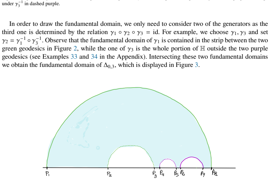
Pith reviewed 2026-05-14 20:39 UTC · model grok-4.3

classification 🧮 math.GT math-phmath.MP
keywords higher Teichmuller spacebordered cusped Teichmuller spacechewing-gum movecandle cakesnake calculusamalgamationFock-Goncharov coordinatesRiemann surfaces with boundary
0
0 comments X

The pith

Colliding boundary components on a Riemann surface produce the bordered cusped Teichmuller space as a confluent limit via the chewing-gum move.

A machine-rendered reading of the paper's core claim, the machinery that carries it, and where it could break.

The lecture notes illustrate how the classical Teichmuller space of hyperbolic surfaces with boundary extends to higher-rank versions through explicit combinatorial constructions. They show that when two boundary components collide, a chewing-gum move on the underlying fat-graph yields a bordered cusped Teichmuller space, realized geometrically as a candle cake. From the Fock-Goncharov viewpoint, the same move acts as the inverse of amalgamation and is expressed through snake calculus on transport matrices in PSL_n(R). The goal is to make these abstract constructions concrete with examples rather than formal proofs, so that the relations among shear coordinates, snake variables, and cusped limits become directly computable.

Core claim

The bordered cusped Teichmuller space arises as the confluent limit obtained when two boundary components in a Riemann surface collide under the chewing-gum move; the resulting object is a candle cake whose combinatorial description is given by the inverse of amalgamation in the snake calculus for PSL_n(R) transport matrices.

What carries the argument

The chewing-gum move on fat-graphs, which merges two boundaries into a single cusp-like structure (candle cake) and inverts amalgamation while preserving the snake calculus relations on PSL_n(R) matrices.

If this is right

  • Shear coordinates on the fat-graph extend directly to the cusped case, allowing the same combinatorial formulas to describe both classical and higher Teichmuller spaces.
  • Snake calculus supplies an explicit matrix representation of the monodromy that remains well-defined after the chewing-gum operation.
  • Amalgamation and its inverse become concrete operations that can be iterated to build surfaces with arbitrary numbers of cusps and boundaries.
  • The constructions remain computationally tractable because they rely only on local moves and matrix multiplications rather than global analytic data.

Where Pith is reading between the lines

These are editorial extensions of the paper, not claims the author makes directly.

  • The same chewing-gum construction could be tested on surfaces with more than two colliding boundaries to produce higher-codimension cusped strata.
  • Because snake calculus is tied to cluster-algebra structures, the candle-cake limit might induce a natural degeneration on the associated cluster variety.
  • The explicit examples in the notes suggest that similar confluent limits could be defined for other higher Teichmuller spaces attached to different Lie groups beyond PSL_n(R).

Load-bearing premise

The chewing-gum move on the fat-graph correctly encodes the confluent limit of colliding boundaries and serves as the exact inverse of amalgamation in the higher Teichmuller setting.

What would settle it

An explicit computation, for a once-punctured torus or four-holed sphere, showing that the shear or snake coordinates obtained after applying the chewing-gum move fail to satisfy the expected Poisson relations or do not reproduce the known dimension and structure of the bordered cusped space.

Figures

Figures reproduced from arXiv: 2605.12572 by Benedetta Facciotti, Marta Mazzocco, Nikita Nikolaev.

Figure 1
Figure 1. Figure 1: The invariant axis of 𝛾1 in yellow, of 𝛾2 in blue and of 𝛾3 in red [PITH_FULL_IMAGE:figures/full_fig_p004_1.png] view at source ↗
Figure 2
Figure 2. Figure 2: The geodesic 𝑔12 is drawn in solid green, its image under 𝛾1 in dashed green. The geodesic 𝑔23 in solid purple, its image under 𝛾 −1 3 in dashed purple. In order to draw the fundamental domain, we only need to consider two of the generators as the third one is determined by the relation 𝛾1 ◦ 𝛾2 ◦ 𝛾3 = id. For example, we choose 𝛾1, 𝛾3 and set 𝛾2 = 𝛾 −1 1 ◦ 𝛾 −1 3 . Observe that the fundamental domain of 𝛾1… view at source ↗
Figure 3
Figure 3. Figure 3: The fundamental domain of Δ0,3 is the region filled in light blue [PITH_FULL_IMAGE:figures/full_fig_p005_3.png] view at source ↗
Figure 4
Figure 4. Figure 4: Gluing the fundamental domain along the green geodesic produces a double funnel with two wedges removed (the areas FEC [PITH_FULL_IMAGE:figures/full_fig_p006_4.png] view at source ↗
Figure 5
Figure 5. Figure 5: The three holed sphere as quotient of H by Δ0,3. The invariant axis of each generator of Δ0,3 gives a closed geodesic which is in the same conjugacy class as the corresponding hole. The green and purple geodesics correspond to the identified boundaries under the quotient [PITH_FULL_IMAGE:figures/full_fig_p006_5.png] view at source ↗
Figure 6
Figure 6. Figure 6: On the left we display the pair of pants cut into two hexagons (on the front, the other on the back). On the right, the [PITH_FULL_IMAGE:figures/full_fig_p008_6.png] view at source ↗
Figure 7
Figure 7. Figure 7: On the left the pair of pants and three infinitely long geodesics triangulating it. On the right their corresponding geodesics [PITH_FULL_IMAGE:figures/full_fig_p009_7.png] view at source ↗
Figure 8
Figure 8. Figure 8: A pair of pants decomposition of Σ3,1. We have denoted in red the geodesics where we cut the surface and in blue the bottle neck geodesic where we chop off the funnel [PITH_FULL_IMAGE:figures/full_fig_p009_8.png] view at source ↗
Figure 9
Figure 9. Figure 9: The ideal triangulation of a pair of pants. [PITH_FULL_IMAGE:figures/full_fig_p010_9.png] view at source ↗
Figure 10
Figure 10. Figure 10: Several identified triangles by the action of the Fuchsian group on the ideal triangulation of a pair of pants. [PITH_FULL_IMAGE:figures/full_fig_p010_10.png] view at source ↗
Figure 11
Figure 11. Figure 11: Proof of Lemma 4. By the action of P𝑆𝐿(2, R), we place the first boundary of un-known length on the imaginary axis, starting at 𝑖 (dashed magenta). Select the unique geodesic (dashed yellow) orthogonal to the imaginary axis in 𝑖. Fix a point 𝑧0 on the dashed yellow geodesic in such a way that the segment of extrema 𝑖 and 𝑧0 has known length 𝑎. Then we take the unique geodesic (dashed green) orthogonal to … view at source ↗
Figure 12
Figure 12. Figure 12: The duality between ideal triangulation (given by the black, blue and green geodesics) and fat-graph in the case of a pair [PITH_FULL_IMAGE:figures/full_fig_p012_12.png] view at source ↗
Figure 13
Figure 13. Figure 13: The orientation on the fat-graph is dictated by the orientation on the ideal triangulation. Going along an edge in the [PITH_FULL_IMAGE:figures/full_fig_p013_13.png] view at source ↗
Figure 14
Figure 14. Figure 14: On the left, the three bottle neck geodesics drawn in the fat-graph, on the right the three edges of the fatgraph and their [PITH_FULL_IMAGE:figures/full_fig_p013_14.png] view at source ↗
Figure 15
Figure 15. Figure 15: Fat graph of Σ0,4. The associated shear coordinates are labeled by 𝑠1, 𝑠2, 𝑠3 and 𝑝1, 𝑝2, 𝑝3. The fundamental group is generated by the 4 loops 𝛾1 in yellow, 𝛾2 in cyan, 𝛾3 in green and 𝛾4 in pink. Note that 𝛾1𝛾2𝛾3𝛾4 = 1. We denote by 𝑠1, 𝑠2, 𝑠3, 𝑝1, 𝑝2, 𝑝3 the shear coordinates associated to the edges of the fat-graph, where the notation distinguishes between edges that go between different vertices and … view at source ↗
Figure 16
Figure 16. Figure 16: On the left we have the initial surface and a closed blue geodesic. On the center, the boundaries start colliding, so that the [PITH_FULL_IMAGE:figures/full_fig_p017_16.png] view at source ↗
Figure 17
Figure 17. Figure 17: On the left we have the initial fat-graph and two closed geodesics in yellow and blue. On the center, the edge labeled by [PITH_FULL_IMAGE:figures/full_fig_p018_17.png] view at source ↗
Figure 18
Figure 18. Figure 18: On the left, the yellow region corresponds to the finite part of a pair of pants. On the right we identify the two purple [PITH_FULL_IMAGE:figures/full_fig_p019_18.png] view at source ↗
Figure 19
Figure 19. Figure 19: On the right, we have two infinitely winding geodesics in green and in black that triangulate the surface. On the left, we [PITH_FULL_IMAGE:figures/full_fig_p019_19.png] view at source ↗
Figure 20
Figure 20. Figure 20: On the left, the ideal triangulation in H and its dual fat-graph which is the same as the one on the right, namely, the fat-graph obtained in [PITH_FULL_IMAGE:figures/full_fig_p020_20.png] view at source ↗
Figure 21
Figure 21. Figure 21: Two horocycles, one at infinity in cyan and one at ˜𝑞 [PITH_FULL_IMAGE:figures/full_fig_p020_21.png] view at source ↗
Figure 22
Figure 22. Figure 22: A generic geodesic (in blue) circling a hole. [PITH_FULL_IMAGE:figures/full_fig_p022_22.png] view at source ↗
Figure 23
Figure 23. Figure 23: The candle cake corresponding to a sphere with three boundaries one of which carries two bordered cusps. [PITH_FULL_IMAGE:figures/full_fig_p023_23.png] view at source ↗
Figure 24
Figure 24. Figure 24: Fat graph of Σ0,3,2. The associated shear coordinates are labeled by 𝑠1, 𝑠2, 𝑠3, 𝑘1, 𝑘2, 𝑝1, 𝑝2. The lamination is composed by two loops around the two boundaries with no bordered cusps and five geodesic arcs denoted by 𝑎, 𝑏, 𝑐, 𝑑, 𝑒 [PITH_FULL_IMAGE:figures/full_fig_p024_24.png] view at source ↗
Figure 25
Figure 25. Figure 25: The triple of transport matrices on the oriented triangle [PITH_FULL_IMAGE:figures/full_fig_p025_25.png] view at source ↗
Figure 27
Figure 27. Figure 27: The triangle graph △3 and its lines and planes. To find lines and planes, we use the formula 𝐹 (1) 3−𝑎 ∩ 𝐹 (2) 3−𝑏 ∩ 𝐹 (3) 3−𝑐 where the lines 𝜆𝑎𝑏𝑐 correspond to 𝑎 + 𝑏 + 𝑐 = 2 and the planes 𝜋𝑎𝑏𝑐 to 𝑎 + 𝑏 + 𝑐 = 1. For the flags of Example 14, we obtain: 𝜆002 = ⟨𝑒1 + 𝛼𝑒2 + 𝛽𝑒3⟩, 𝜆101 = ⟨𝛾𝑒1 + (𝛼𝛾 − 𝛽)𝑒2⟩, 𝜆200 = ⟨𝑒1⟩, 𝜆110 = ⟨𝑒2⟩, 𝜆020 = ⟨𝑒3⟩, 𝜆011 = ⟨𝑒2 + 𝛾𝑒3⟩, 𝜋100 = ⟨𝑒1, 𝑒2⟩, 𝜋010 = ⟨𝑒3, 𝑒2⟩, 𝜋001 = ⟨𝑒1… view at source ↗
Figure 28
Figure 28. Figure 28: For 𝑛 = 3, from left to right: tessellation of △123, barycentric coordinates for vertices of the tessellation and centers of the tiles, configuration of subspaces with the gray triangles (and one white triangle surrounded by them). over their sides. Notice that the upward gray and downward white triangles give precisely the 𝑛 − 1 tessellation of a triangle connecting {𝜆(𝑛−1)00, 𝜆0(𝑛−1)0, 𝜆00(𝑛−1) }. Defin… view at source ↗
Figure 29
Figure 29. Figure 29: Segments of two oppositely oriented snakes. The vertices of the gray triangle correspond to 3 coplanar lines [PITH_FULL_IMAGE:figures/full_fig_p032_29.png] view at source ↗
Figure 30
Figure 30. Figure 30: Take any 𝑤1 ∈ 𝜆1 and denote its end point by 𝑤1 with abuse of notation, then consider the blue line that is parallel to 𝜆3 through 𝑤1. This blue line intersects 𝜆2 at a point 𝑤2. Take 𝑤2 ∈ 𝜆2 to be the vector whose end point is 𝑤2. In this case 𝑤1 − 𝑤2 ∈ 𝜆3. 12 12 3 w de Is as As Wz Pez WL W _Wz With 13 12 13 12 Witweeds Wz Wi dy Wi as Withst tz 12 Wz 4 We 1 [PITH_FULL_IMAGE:figures/full_fig_p033_30.png] view at source ↗
Figure 31
Figure 31. Figure 31: Take any 𝑤1 ∈ 𝜆1 and denote its end point by 𝑤1 with abuse of notation, then consider the blue line that is orthogonal to 𝜆3 through 𝑤1. This blue line intersects 𝜆2 at a point 𝑤2. Take 𝑤2 ∈ 𝜆2 to be the vector whose end point is 𝑤2. In this case 𝑤1 + 𝑤2 ∈ 𝜆3. Therefore, a snake inductively determines a basis of R 𝑛 up to global rescaling: Once the first vector is chosen, iteratively applying the rule, th… view at source ↗
Figure 32
Figure 32. Figure 32: From left to right, elementary snake moves I,II and III mapping [PITH_FULL_IMAGE:figures/full_fig_p035_32.png] view at source ↗
Figure 33
Figure 33. Figure 33: Sequence of snake moves factorizing 𝑇˜ 1 for 𝑛 = 3. At step 2, the tessellation’s only inner vertex of barycentric coordinates (1, 1, 1) labels the Fock-Goncharov variable 𝑍111. At step 4, the 𝜕-snake runs counterclockwise and an 𝑆 matrix is needed. 5.5 Fock Goncharov coordinates as triple ratios As mentioned after formula (33), there is a Fock-Goncharov variable for every white triangle. Each such white … view at source ↗
Figure 34
Figure 34. Figure 34: On the left, we highlight a white triangle and its three adjacent gray ones. On the right we display the isomorphic [PITH_FULL_IMAGE:figures/full_fig_p036_34.png] view at source ↗
Figure 35
Figure 35. Figure 35: Fock-Goncharov variables 𝑍𝛼 for PPGL2 (R) (△123 ) on the left and PPGL3 (R) (△123 ) on the right. Blue variables are associated with moves II and red ones with side pinnings. As a whole, they are in bijection with the tessellation’s vertices except 1, 2, 3. Definition 10 The transport matrices 𝑇1, 𝑇2, 𝑇3 are the following PGL𝑛(R) matrices [PITH_FULL_IMAGE:figures/full_fig_p038_35.png] view at source ↗
Figure 36
Figure 36. Figure 36: On the left two adjacent triangles, on the right, the separated triangles with labeled vertices. [PITH_FULL_IMAGE:figures/full_fig_p040_36.png] view at source ↗
Figure 37
Figure 37. Figure 37: The fat graph of the cylinder with two bordered cusps on one boundary and its dual triangulation. The generating paths [PITH_FULL_IMAGE:figures/full_fig_p041_37.png] view at source ↗
Figure 38
Figure 38. Figure 38: On the left, The fat graph of the cylinder with two bordered cusps on one boundary and its dual triangulation with one [PITH_FULL_IMAGE:figures/full_fig_p042_38.png] view at source ↗
Figure 39
Figure 39. Figure 39: On the left, the amalgamation process of [PITH_FULL_IMAGE:figures/full_fig_p043_39.png] view at source ↗
Figure 40
Figure 40. Figure 40: The three triangles as in Figure [PITH_FULL_IMAGE:figures/full_fig_p044_40.png] view at source ↗
Figure 41
Figure 41. Figure 41: The fat graph of a sphere with four boundary components, its dual triangulation and the loops corresponding the [PITH_FULL_IMAGE:figures/full_fig_p047_41.png] view at source ↗
Figure 42
Figure 42. Figure 42: Points 𝑃 ′ , 𝑄′ on the absolute [PITH_FULL_IMAGE:figures/full_fig_p049_42.png] view at source ↗
Figure 43
Figure 43. Figure 43: The hyperbolic circle of center 𝑖 and radius 2. 𝑐𝑧𝑧 + 𝛼𝑧 + 𝛼𝑧 + 𝑑 = 0 where 𝛼 is a complex constant, and 𝑐, 𝑑 are real numbers. If 𝑐 = 0, the cline is a line, while for 𝑐 ≠ 0 it is a circle of center 𝑧0 and radius 𝑟 where 𝑧0 =  − ℜ𝛼 𝑐 , ℑ𝛼 𝑐  , 𝑟 = √︂ 𝛼𝛼 𝑐 2 Definition 13 A horocycle is a Euclidean circle in H tangent to the absolute. There are two types of horocycles in H: the ones based at infinity, w… view at source ↗
Figure 44
Figure 44. Figure 44: On the left, a given a vertical geodesic [PITH_FULL_IMAGE:figures/full_fig_p052_44.png] view at source ↗
Figure 45
Figure 45. Figure 45: The action of the elliptic element 𝛾𝑒. 5.12.2 Action of parabolic elements For parabolic elements, any horocycle at the fixed point is invariant. Indeed, we can always apply a transformation in P𝑆𝐿(2, R) to map a parabolic element to one of the form 𝛾𝑝 (𝑧) = 𝑧 + 𝑟, where 𝑟 ∈ R. Horocycles based at the fixed point ∞ are horizontal lines which are simply translated under the action of 𝛾𝑝. This shows that pa… view at source ↗
Figure 46
Figure 46. Figure 46: Various clines through [PITH_FULL_IMAGE:figures/full_fig_p054_46.png] view at source ↗
Figure 47
Figure 47. Figure 47: The action of 𝛾1. left 2q1 right left right 3q1 right left 32q rangle [PITH_FULL_IMAGE:figures/full_fig_p056_47.png] view at source ↗
Figure 48
Figure 48. Figure 48: The action of 𝛾3. the dashed purple one. A fundamental domain for the hyperbolic element 𝛾3 (𝑧) is the portion of the upper half plane above the solid and dashed purple geodesics in [PITH_FULL_IMAGE:figures/full_fig_p056_48.png] view at source ↗
read the original abstract

The aim of these lecture notes, based on lectures given by the second author at the CIME school in Cetraro, is to illustrate a range of ideas surrounding higher Teichmuller spaces of Riemann surfaces with marked boundaries through explicit and computationally tractable examples. After reviewing the classical Teichmuller space of hyperbolic Riemann surfaces with boundary and its combinatorial description in terms of Thurston shear coordinates on a fat-graph, we explain how the bordered cusped Teichmuller space arises as a confluent limit when two boundary components in the Riemann surface collide via the so-called chewing-gum move giving rise to a candle cake. We then revisit these constructions from the Fock-Goncharov perspective, explaining snake calculus for transport matrices in PSL_n(R) and explain how the chewing gum move is the inverse of amalgamation. Rather than focusing on formal proofs, our goal is to illustrate the underlying theorems and constructions in a concrete and intuitive way.

Editorial analysis

A structured set of objections, weighed in public.

Desk editor's note, referee report, simulated authors' rebuttal, and a circularity audit. Tearing a paper down is the easy half of reading it; the pith above is the substance, this is the friction.

Referee Report

0 major / 2 minor

Summary. These lecture notes review the classical Teichmüller space of hyperbolic Riemann surfaces with boundary and its combinatorial description via Thurston shear coordinates on fat-graphs, then explain how the bordered cusped Teichmüller space arises as a confluent limit when two boundary components collide under the chewing-gum move (producing a candle cake). The notes revisit the constructions from the Fock-Goncharov viewpoint, introducing snake calculus for transport matrices in PSL_n(R) and showing that the chewing-gum move inverts amalgamation. The emphasis is on concrete, computationally tractable examples rather than formal proofs.

Significance. The notes supply accessible, example-driven illustrations of established constructions in classical and higher Teichmüller theory, including the confluent-limit description of bordered cusped spaces and the relation between chewing-gum moves and Fock-Goncharov amalgamation. Such expository material with explicit combinatorial and matrix-level pictures can help readers connect abstract theorems to concrete computations.

minor comments (2)
  1. [Abstract] The abstract introduces the term 'candle cake' without a brief parenthetical gloss; adding one sentence in the introduction would clarify the geometric picture for readers unfamiliar with the construction.
  2. A short list of key references to the original Fock-Goncharov papers and to the relevant results on amalgamation would help readers locate the theorems being illustrated.

Simulated Author's Rebuttal

0 responses · 0 unresolved

We thank the referee for their positive summary, recognition of the expository value of the notes, and recommendation to accept. The manuscript is intended as accessible lecture notes illustrating concrete examples rather than a formal research paper, and we are pleased this approach was appreciated.

Circularity Check

0 steps flagged

No significant circularity

full rationale

The manuscript consists of expository lecture notes illustrating established constructions in classical and higher Teichmüller theory. The chewing-gum move is described as producing the bordered cusped Teichmüller space as a confluent limit and as the inverse of Fock-Goncharov amalgamation, but these relations are presented as known results from the literature rather than new derivations whose validity depends on self-referential steps, fitted parameters, or unverified self-citations. No load-bearing claim reduces by construction to the paper's own inputs; the text explicitly states its goal is to illustrate underlying theorems concretely without formal proofs.

Axiom & Free-Parameter Ledger

0 free parameters · 2 axioms · 0 invented entities

The notes build entirely on established Teichmuller theory and Fock-Goncharov frameworks with no new parameters or entities introduced.

axioms (2)
  • standard math Standard properties of Teichmuller spaces for Riemann surfaces with boundary and Thurston shear coordinates
    Reviewed as background for the classical case before introducing the chewing-gum construction.
  • domain assumption Fock-Goncharov theory for higher Teichmuller spaces including snake calculus and amalgamation
    Used to reinterpret the chewing-gum move as the inverse of amalgamation.

pith-pipeline@v0.9.0 · 5463 in / 1207 out tokens · 51801 ms · 2026-05-14T20:39:59.604490+00:00 · methodology

discussion (0)

Sign in with ORCID, Apple, or X to comment. Anyone can read and Pith papers without signing in.

Reference graph

Works this paper leans on

21 extracted references · 21 canonical work pages · 1 internal anchor

  1. [1]

    Burger, M., Iozzi, A., Wienhard, A.: Surface group representations with maximal Toledo invariant. C. R. Math. Acad. Sci. Paris336(5), 387–390 (2003)

  2. [2]

    Chekhov, L., Fock, V.V.: A quantum Teichm¨ uller space. Theor. Math. Phys.120, 1245–1259 (1999)

  3. [3]

    Nonlinearity31(1), 54–107 (2018)

    Chekhov, L.O., Mazzocco, M.: Colliding holes in Riemann surfaces and quantum cluster algebras. Nonlinearity31(1), 54–107 (2018)

  4. [4]

    Chekhov, L.O., Mazzocco, M., Rubtsov, V.: Painlev´e monodromy manifolds, decorated character varieties, and cluster algebras. Int. Math. Res. Not. IMRN2017(24), 7639–7691 (2017). doi: 10.1093/imrn/rnw219

  5. [5]

    Regularity and Inferential Theories of Causation

    Chekhov, L.O., Mazzocco, M., Rubtsov, V.: Algebras of quantum monodromy data and decorated character varieties. In: Dancer, A., Garc´ıa-Prada, O., Kirwan, F. (eds.) Geometry and Physics: A Festschrift in honour of Nigel Hitchin, Vol. I, pp. 39–68. Oxford University Press, Oxford (2018). doi: 10.1093/oso/9780198802013.003.0003

  6. [6]

    In: Papadopoulos, A

    Chekhov, L.O., Penner, R.C.: On quantizing Teichm¨ uller and Thurston theories. In: Papadopoulos, A. (ed.) Handbook of Teichm¨ uller Theory, Vol. I. IRMA Lect. Math. Theor. Phys., vol. 11, pp. 579–645. European Mathematical Society, Z¨ urich (2007)

  7. [7]

    Dal Martello, D., Mazzocco, M.: Generalized double affine Hecke algebras, their representations, and higher Teichm¨ uller theory. Adv. Math.450, Paper No. 109763 (2024). doi: 10.1016/j.aim.2024.109763

  8. [8]

    Facciotti, B., Mazzocco, M., Nikolaev, N.: Decorated local systems and character varieties.https://arxiv.org/abs/ 2603.18842(2026) Chewing gums, snakes and candle cakes. 57

  9. [9]

    Fock, V.V.: Combinatorial description of the moduli space of projective structures.https://arxiv.org/abs/hep-th/ 9312193

  10. [10]

    Fock, V.V.: Dual Teichm¨ uller spaces.https://arxiv.org/abs/dg-ga/9702018

  11. [11]

    Fock, V.V., Goncharov, A.: Moduli spaces of local systems and higher Teichm¨ uller theory. Publ. Math. Inst. Hautes´Etudes Sci.103, 1–211 (2006)

  12. [12]

    Goldman, W.M.: Topological components of spaces of representations. Invent. Math.93(3), 557–607 (1988)

  13. [13]

    org/abs/1904.10491(2022)

    Goncharov, A., Shen, L.: Quantum geometry of moduli spaces of local systems and representation theory.https://arxiv. org/abs/1904.10491(2022)

  14. [14]

    Topology31(3), 449–473 (1992)

    Hitchin, N.J.: Lie groups and Teichm¨ uller space. Topology31(3), 449–473 (1992)

  15. [15]

    Kashaev, R.M.: Quantization of Teichm¨ uller spaces and the quantum dilogarithm. Lett. Math. Phys.43, 105–115 (1998)

  16. [16]

    Labourie, F.: Anosov flows, surface groups and curves in projective space. Invent. Math.165, 51–114 (2006)

  17. [17]

    Magnus, W.: Rings of Fricke characters and automorphism groups of free groups. Math. Z.170, 91–103 (1980)

  18. [18]

    Academic Press, San Diego (1991)

    Nash, C.: Differential Topology and Quantum Field Theory. Academic Press, San Diego (1991)

  19. [19]

    Penner, R.C.: The decorated Teichm¨ uller space of Riemann surfaces. Comm. Math. Phys.113, 299–339 (1988)

  20. [20]

    Lecture notes for course MA448, University of Warwick (2010)

    Series, C., Maloni, S.: Hyperbolic geometry. Lecture notes for course MA448, University of Warwick (2010). https://warwick.ac.uk/fac/sci/maths/people/staff/caroline_series/hyperbolic_geometry_ma448_ lecture_notes.pdf

  21. [21]

    In: Sirakov, B., de Souza, P.N., Viana, M

    Wienhard, A.: An invitation to higher Teichm¨ uller theory. In: Sirakov, B., de Souza, P.N., Viana, M. (eds.) Proceedings of the International Congress of Mathematicians—Rio de Janeiro 2018, Vol. II: Invited Lectures, pp. 1013–1039. World Scientific Publishing, Hackensack, NJ (2018)