Recognition: no theorem link
The inverse curve shortening flow on the hyperbolic plane
Pith reviewed 2026-05-15 01:42 UTC · model grok-4.3
The pith
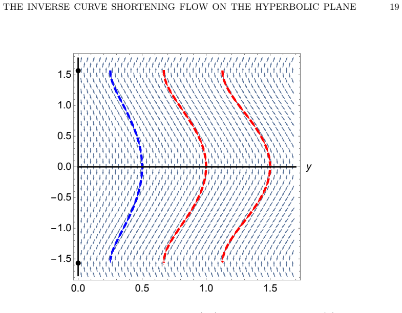
In the hyperbolic plane, all parabolic solitons of the inverse curve shortening flow are graphs over the y-axis and all conformal solitons are graphs over the x-axis in the upper half-plane model.
A machine-rendered reading of the paper's core claim, the machinery that carries it, and where it could break.
Core claim
We classify all solitons with respect to parabolic and conformal vector fields of H^2. In the upper half-plane model of H^2, we prove that parabolic solitons are all graphs on the y-axis, whereas conformal solitons are graphs on the x-axis. We study the concavity of these solitons and when they approach the coordinate axes.
What carries the argument
The upper half-plane model of H^2, which converts the soliton equation for parabolic and conformal vector fields into the condition that the curve is a graph over one of the coordinate axes.
If this is right
- Parabolic solitons are exactly the graphs over the y-axis.
- Conformal solitons are exactly the graphs over the x-axis.
- The concavity of each family can be computed directly from the soliton equation.
- The graphs approach the coordinate axes under explicit conditions on their defining functions.
Where Pith is reading between the lines
- The explicit graphical form may allow direct construction of ancient or eternal solutions to the flow.
- The same reduction technique could be tested on other Killing fields or on the sphere and Euclidean plane for comparison.
- Concavity results may translate into curvature estimates that control singularity formation for the flow.
Load-bearing premise
The inverse curve shortening flow is assumed to be well-defined on the curves considered, and the classification is restricted to parabolic and conformal vector fields.
What would settle it
A single explicit example of a parabolic soliton in the upper half-plane model that fails to be a graph over the y-axis would disprove the classification.
Figures


read the original abstract
We study the inverse curve shortening flow in the hyperbolic plane $\h^2$. We classify all solitons with respect to parabolic and conformal vector fields of $\h^2$. In the upper half-plane model of $\h^2$, we prove that parabolic solitons are all graphs on the $y$-axis, whereas conformal solitons are graphs on the $x$-axis. We study the concavity of these solitons and when they approach the coordinate axes.
Editorial analysis
A structured set of objections, weighed in public.
Referee Report
Summary. The paper studies the inverse curve shortening flow in the hyperbolic plane H². It classifies all solitons with respect to parabolic and conformal vector fields of H². In the upper half-plane model, it proves that parabolic solitons are graphs over the y-axis while conformal solitons are graphs over the x-axis, and it examines their concavity and asymptotic approach to the coordinate axes.
Significance. If the classification holds, the explicit graph representations of solitons under these symmetries provide concrete geometric information that can inform analysis of the flow's long-time behavior and singularity formation in hyperbolic geometry. The direct derivation from the flow equation (without fitted parameters) is a strength.
major comments (2)
- [§3] §3, Theorem 3.1: the step establishing that parabolic solitons must be graphs over the y-axis requires an explicit verification that the transversality condition to the parabolic vector field is preserved; the current argument appears to assume this without a maximum-principle estimate or boundary analysis at infinity.
- [§4] §4, Eq. (4.3): the ODE for conformal solitons yields graphs over the x-axis only after imposing the conformal Killing condition; a short remark confirming that no other solutions exist outside this ansatz would strengthen the completeness of the classification.
minor comments (2)
- [Abstract] The abstract states the main results but does not reference the theorem numbers; adding these would improve navigation.
- [§2] Notation for the hyperbolic metric and the precise definitions of parabolic versus conformal vector fields could be collected in a preliminary section for easier reference.
Simulated Author's Rebuttal
We thank the referee for the careful reading of our manuscript and the positive recommendation for minor revision. We address each major comment below and have revised the paper accordingly to strengthen the arguments.
read point-by-point responses
-
Referee: [§3] §3, Theorem 3.1: the step establishing that parabolic solitons must be graphs over the y-axis requires an explicit verification that the transversality condition to the parabolic vector field is preserved; the current argument appears to assume this without a maximum-principle estimate or boundary analysis at infinity.
Authors: We agree that an explicit verification of the preservation of the transversality condition is required for rigor. In the revised version of the manuscript, we have added a maximum-principle argument in the proof of Theorem 3.1 showing that the angle between the curve and the parabolic vector field remains strictly positive. This is supplemented by an analysis at infinity that uses the asymptotic behavior established later in the section to rule out tangency or crossing. These additions confirm that the solitons are graphs over the y-axis without assuming the condition a priori. revision: yes
-
Referee: [§4] §4, Eq. (4.3): the ODE for conformal solitons yields graphs over the x-axis only after imposing the conformal Killing condition; a short remark confirming that no other solutions exist outside this ansatz would strengthen the completeness of the classification.
Authors: We thank the referee for this suggestion. We have inserted a short remark immediately after Equation (4.3) explaining that the conformal Killing condition is imposed because only conformal vector fields preserve the hyperbolic metric up to scale and thus qualify as symmetries for the inverse curve shortening flow. By the standard classification of conformal Killing fields on H², no other vector fields satisfy the soliton equation outside this ansatz. revision: yes
Circularity Check
No significant circularity
full rationale
The paper derives the classification of solitons for the inverse curve shortening flow directly from the soliton PDE in the upper half-plane model of H^2. Parabolic solitons are proved to be graphs over the y-axis and conformal solitons over the x-axis by solving the flow equation with respect to the given vector fields. No load-bearing step reduces by construction to a fitted parameter, self-citation, or imported ansatz; the argument is self-contained in the model's explicit coordinate computations and does not rely on external uniqueness theorems or prior author results as premises.
Axiom & Free-Parameter Ledger
axioms (2)
- domain assumption The inverse curve shortening flow is well-defined on immersed curves in H^2
- ad hoc to paper Parabolic and conformal vector fields are the relevant symmetry fields for soliton classification
Reference graph
Works this paper leans on
-
[1]
B. D. Allen, Non-compact solutions to inverse mean curvature flow in hyperbolic space. Ph.D. thesis, University of Tennessee, Knoxville, 2016
work page 2016
- [2]
- [3]
- [4]
-
[5]
B. Choi, P. Daskalopoulos, Evolution of non-compact hypersurfaces by inverse mean curvature. Duke Math. J. 170 (2021), 2755–2803
work page 2021
- [6]
- [7]
-
[8]
M. E. Gage, Curve shortening makes convex curves circular. Invent. Math. 76 (1984), 357–364
work page 1984
-
[9]
Gerhardt, Flow of nonconvex hypersurfaces into spheres
C. Gerhardt, Flow of nonconvex hypersurfaces into spheres. J. Differential Geom. 32 (1990), 299–314
work page 1990
-
[10]
C. Gerhardt, Curvature problems. Ser. Geom. Topol. vol. 39. International Press, Boston. 2006
work page 2006
-
[11]
Gerhardt, Inverse curvature flows in hyperbolic space
C. Gerhardt, Inverse curvature flows in hyperbolic space. J. Differential Geom. 89 (2011), 487–527
work page 2011
-
[12]
G. Huisken, T. Ilmanen, The inverse mean curvature flow and the Riemannian Penrose in- equality. J. Differential Geom. 59 (2001), 353–437
work page 2001
-
[13]
P.-K. Hung, M.-T. Wang, Inverse mean curvature flows in the hyperbolic 3-space revisited. Calc. Var. Partial Differential Equations 54 (2015), 119–126
work page 2015
-
[14]
D. Kim, J. Pyo, Remarks on solitons for inverse mean curvature flow. Math. Nach. 293 (2020), 2363–2369
work page 2020
-
[15]
H. Li, Y. Wei, On inverse mean curvature flow in Schwarzschild space and Kottler space. Calc. Var. Partial Differential Equations 56 (2017), no. 3, Paper No. 62. 22 IVAN KRZNARI ´C AND RAFAEL L ´OPEZ
work page 2017
-
[16]
Lu, Inverse curvature flow in anti-de Sitter-Schwarzschild manifold
S. Lu, Inverse curvature flow in anti-de Sitter-Schwarzschild manifold. Comm. Anal. Geom. 27 (2019), 465–489
work page 2019
-
[17]
L. Mari, J. R. Oliveira, A. Savas-Halilaj, R. Sodr´ e de Sena, Conformal solitons for the mean curvature flow in hyperbolic space. Ann. Glob. Anal. Geom. 65 (2024), 19
work page 2024
-
[18]
G. S. Neto, V. Silva, Classification of ruled surfaces as homothetic self-similar solutions of the inverse mean curvature flow in the Lorentz-Minkowski 3-space. Bull. Braz. Math. Soc. New Ser. 54, Art. 48 (2023)
work page 2023
-
[19]
Pipoli, Inverse mean curvature flow in quaternionic hyperbolic space
G. Pipoli, Inverse mean curvature flow in quaternionic hyperbolic space. Atti Accad. Naz. Lincei Rend. Lincei Mat. Appl. 29 (2018), 153–171
work page 2018
-
[20]
Pipoli, Inverse mean curvature flow in complex hyperbolic space
G. Pipoli, Inverse mean curvature flow in complex hyperbolic space. Ann. Scient. `Ec. Norm. Sup. 52 (2019), 1107–1135
work page 2019
-
[21]
Scheuer, The inverse mean curvature flow in warped cylinders of non-positive radial curva- ture
J. Scheuer, The inverse mean curvature flow in warped cylinders of non-positive radial curva- ture. Adv. Math. 306 (2017), 1130–1163
work page 2017
-
[22]
Zhou, Inverse mean curvature flows in warped product manifolds
H. Zhou, Inverse mean curvature flows in warped product manifolds. J. Geom. Anal. 28 (2018), 1749–1772. Faculty of Economics and Business. University of Zagreb Email address:ikrznaric@efzg.hr Departamento de Geometr´ıa y Topolog´ıa Universidad de Granada 18071 Granada, Spain Email address:rcamino@ugr.es
work page 2018
discussion (0)
Sign in with ORCID, Apple, or X to comment. Anyone can read and Pith papers without signing in.