arxiv: 2605.14405 · v1 · submitted 2026-05-14 · 💻 cs.LG · math.DS

Recognition: 2 theorem links

· Lean Theorem

Watch your neighbors: Training statistically accurate chaotic systems with local phase space information

Joon-Hyuk Ko , Andrus Giraldo , Deok-Sun Lee

Authors on Pith no claims yet

Pith reviewed 2026-05-15 02:32 UTC · model grok-4.3

classification 💻 cs.LG math.DS

keywords chaotic dynamicssurrogate modelingmaximum mean discrepancyphase space coveringJacobian accuracydata-driven discoverystatistical fidelitylocal pushforwards

0 comments

The pith

A surrogate model for chaotic dynamics is trained by matching pushforward distributions of local phase space coverings under maximum mean discrepancy to achieve both accurate Jacobians and long-term statistics.

A machine-rendered reading of the paper's core claim, the machinery that carries it, and where it could break.

The paper introduces a training framework that covers a chaotic attractor locally in phase space and minimizes the maximum mean discrepancy between the distributions obtained by pushing these coverings forward under the surrogate dynamics versus the ground-truth dynamics. This simultaneously targets accurate local expansion and contraction rates captured by the Jacobian while preserving global statistical properties of the attractor. Prior approaches had optimized either for Jacobian fidelity or for statistical reproduction but not both at once. The resulting surrogates show markedly better Jacobian accuracy in experiments without sacrificing competitiveness on statistical benchmarks. The method relies on the local coverings being sufficiently representative so that distribution matching enforces the desired local linearization properties.

Core claim

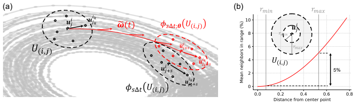
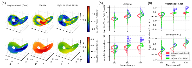
We construct a local covering of a chaotic attractor in phase space and analyze the expansion and contraction of these coverings under the dynamics. The surrogate model is trained by minimizing the maximum mean discrepancy between the pushforward distributions of the coverings under the surrogate and ground-truth dynamics, yielding models with significantly improved Jacobian accuracy while remaining competitive with state-of-the-art statistically accurate dynamics learning methods.

What carries the argument

Local coverings of the attractor whose pushforward distributions are aligned via MMD minimization between surrogate and true dynamics.

If this is right

Surrogate models will exhibit reduced sensitivity to initial-condition perturbations because local expansion rates are better preserved.
Long-term statistical reproduction will be maintained without the usual trade-off against local linear accuracy.
The framework can be applied to any data-driven dynamics learner that can evaluate or differentiate the surrogate map.
Training can proceed with shorter trajectory segments since the method operates on local distributions rather than full long-horizon rollouts.

Where Pith is reading between the lines

These are editorial extensions of the paper, not claims the author makes directly.

The same covering-based MMD objective might stabilize training of recurrent models for other sensitive systems such as fluid flows or biological oscillators.
Adaptive choice of covering density according to local Lyapunov exponents could further tighten the Jacobian match.
The approach suggests a general route for enforcing local stability constraints in generative models of dynamical systems without explicit Jacobian regularization terms.

Load-bearing premise

The selected local coverings must be representative of the full attractor so that matching their pushforward distributions enforces accurate Jacobians without introducing new biases in the learned dynamics.

What would settle it

A concrete falsifier would be finding that a model trained this way achieves low MMD on the pushforwards yet its computed Jacobians deviate substantially from the true system's Jacobians on held-out points sampled from the attractor.

Figures

Figures reproduced from arXiv: 2605.14405 by Andrus Giraldo, Deok-Sun Lee, Joon-Hyuk Ko.

**Figure 1.** Figure 1: Schematic of our Neighborhood method. (a) We focus on finite cover of the attractor U(i,j) and regularize training so that the model deforms the cover in the same manner as the ground truth dynamics. (b) We design our cover sets to be annuli to mitigate the effects of noise. Estimating the time-evolution of attractor covers from data Since our dataset consists of discrete trajectory measurements on the cha… view at source ↗

**Figure 2.** Figure 2: Short-term accuracy of the trained models. [PITH_FULL_IMAGE:figures/full_fig_p007_2.png] view at source ↗

**Figure 3.** Figure 3: Long-term statistical accuracy of the trained models. [PITH_FULL_IMAGE:figures/full_fig_p008_3.png] view at source ↗

**Figure 4.** Figure 4: Local behavior of the trained models. (a) Relative error in the vector field (upper row) and the Jacobians (lower row) for models trained on the 3D Lorenz 63 system with 10% noise. (b) Violin plots of the relative vector field and Jacobian errors for the Lorenz 63 system, across all noise strengths. (c) Relative Jacobian error with varying noise strengths for different systems. Lyapunov exponents As a key … view at source ↗

**Figure 5.** Figure 5: Lyapunov exponents of the trained models. [PITH_FULL_IMAGE:figures/full_fig_p014_5.png] view at source ↗

**Figure 6.** Figure 6: Hyperparameter sweep results for DySLIM. The green box indicates the selected hyperpa [PITH_FULL_IMAGE:figures/full_fig_p017_6.png] view at source ↗

**Figure 7.** Figure 7: Hyperparameter sweep results for our Neighborhood method. The green box indicates the [PITH_FULL_IMAGE:figures/full_fig_p018_7.png] view at source ↗

**Figure 8.** Figure 8: Calculation of baseline MMD2 value for the hyperchaotic Chen system. (a) Time evolution of the MMD2 computed between two samples of the chaotic attractor, both evolved using the ground truth dynamics. Note that unlike Fig. 3b, the values do not start from zero as the initial conditions for the two attractor samples are different. (b) Histograms of the ground truth attractor samples at different rollout tim… view at source ↗

read the original abstract

Chaotic systems pose fundamental challenges for data-driven dynamics discovery, as small modeling errors lead to exponentially growing trajectory discrepancies. Since exact long-term prediction is unattainable, it is natural to ask what a good surrogate model for chaotic dynamics is. Prior work has largely focused either on reproducing the Jacobian of the underlying dynamics, which governs local expansion and contraction rates, or on training surrogate models that reproduce the ground-truth dynamics' long-term statistical behavior. In this work, we propose a new framework that aims to bridge these two paradigms by training surrogate dynamics models with accurate Jacobians and long-term statistical properties. Our method constructs a local covering of a chaotic attractor in phase space and analyzes the expansion and contraction of these coverings under the dynamics. The surrogate model is trained by minimizing the maximum mean discrepancy between the pushforward distributions of the coverings under the surrogate and ground-truth dynamics. Experiments show that our method significantly improves Jacobian accuracy while remaining competitive with state-of-the-art statistically accurate dynamics learning methods. Our code is fully available at https://anonymous.4open.science/r/neighborwatch.

Editorial analysis

A structured set of objections, weighed in public.

Desk editor's note, referee report, simulated authors' rebuttal, and a circularity audit. Tearing a paper down is the easy half of reading it; the pith above is the substance, this is the friction.

Desk Editor's Note private letter to a colleague

The paper gives a workable way to train chaotic surrogates by matching pushforward distributions of local attractor patches with MMD, which improves Jacobian accuracy on top of statistical fidelity.

read the letter

The main thing here is a training loop that covers the attractor with small local patches, pushes those patches forward under both the true map and the learned surrogate, and minimizes MMD between the resulting point clouds. This is supposed to pull the surrogate toward correct local expansion rates while still matching the long-term statistics that matter for chaotic systems. The abstract and the stress-test note both point to experiments that show Jacobian gains without falling behind on statistical benchmarks, and the code is released, which is helpful for checking the details. That combination of local covering analysis with distribution matching on the images looks like the actual new piece relative to earlier work that chased only one of the two objectives. The approach is internally consistent and directly targets a real tension in the field. The soft spot is exactly the one the stress-test flags: finite-radius patches mean the pushforward distribution can be matched by nonlinear compensation even if the local linearization (the Jacobian) is systematically off. Nothing in the abstract supplies a theorem that MMD convergence implies Jacobian convergence in the small-radius limit, nor does it show ablations that separate the Jacobian improvement from the statistical term. Without those, the reported gains could be an indirect side effect rather than a direct result of the covering construction. This is for people who build data-driven models of chaotic flows or climate-like systems and want surrogates that respect both local rates and global measures. A reader working on that intersection would get concrete value from the framework and the public code, even if the current evidence leaves the precise mechanism open to verification. I would send it to peer review; the idea is clear enough and the practical goal is relevant enough that referees can sort out the remaining questions on the loss-to-Jacobian link.

Referee Report

2 major / 2 minor

Summary. The paper proposes a framework for training surrogate models of chaotic dynamical systems that aims to achieve both accurate local Jacobians and long-term statistical fidelity. It constructs local coverings of the attractor, analyzes their expansion/contraction under the dynamics, and trains the surrogate by minimizing maximum mean discrepancy (MMD) between the pushforward distributions of these coverings under the surrogate map and the ground-truth dynamics. Experiments are reported to show significantly improved Jacobian accuracy while remaining competitive with state-of-the-art statistically accurate methods.

Significance. If the central claim holds, the work would be significant for data-driven modeling of chaotic systems, as it attempts to bridge the gap between Jacobian-focused and statistics-focused training paradigms. Accurate Jacobians are critical for controlling local expansion rates that drive exponential divergence, while statistical accuracy ensures faithful long-term behavior; a method that reliably delivers both could improve surrogate reliability in applications such as weather forecasting or turbulence modeling. The public code release is a positive factor for reproducibility.

major comments (2)

[Abstract / Method] Abstract and §3 (method description): the central claim that MMD minimization on pushforwards of finite-radius local coverings produces accurate Jacobians is not supported by any theorem or analysis. For positive-radius patches the pushforward distribution depends on the full nonlinear image, so a surrogate can match the empirical distribution (low MMD) while possessing systematically incorrect singular values of the Jacobian, provided higher-order terms compensate inside each patch. No term in the loss explicitly penalizes ||Df(x) − DF(x)|| and no convergence result is given as patch radius → 0.
[Experiments] Experiments section: the reported Jacobian improvements are presented as a direct consequence of the covering construction, yet the manuscript provides no ablation on patch radius, no independent verification that the loss produces Jacobian gains beyond improved global statistics, and no quantitative comparison of Jacobian error norms against baselines that already target statistics. Without these controls the observed gains could be an indirect side-effect rather than evidence for the claimed mechanism.

minor comments (2)

[Method] The description of how the local coverings are chosen and how their radii are selected should be expanded with explicit pseudocode or a dedicated subsection; current presentation leaves the precise construction ambiguous.
[Experiments] Table or figure captions for Jacobian and statistical metrics should include the precise error norms used (e.g., Frobenius norm on Jacobian, specific MMD kernel) and report standard deviations across multiple random seeds.

Simulated Author's Rebuttal

2 responses · 0 unresolved

We thank the referee for the constructive and detailed report. The comments highlight important aspects of the theoretical grounding and experimental validation of our framework. We address each major comment below and outline the revisions we will make.

read point-by-point responses

Referee: [Abstract / Method] Abstract and §3 (method description): the central claim that MMD minimization on pushforwards of finite-radius local coverings produces accurate Jacobians is not supported by any theorem or analysis. For positive-radius patches the pushforward distribution depends on the full nonlinear image, so a surrogate can match the empirical distribution (low MMD) while possessing systematically incorrect singular values of the Jacobian, provided higher-order terms compensate inside each patch. No term in the loss explicitly penalizes ||Df(x) − DF(x)|| and no convergence result is given as patch radius → 0.

Authors: We agree that the manuscript lacks a formal theorem establishing Jacobian convergence as patch radius tends to zero. The method relies on the approximation that sufficiently small patches make the pushforward distribution sensitive primarily to the linear (Jacobian) term, with the MMD objective encouraging matching of local expansion/contraction rates. While higher-order nonlinear terms could theoretically compensate within finite patches, the local covering construction and empirical results indicate that this regularization improves Jacobian fidelity in practice for the systems considered. In the revision we will add a dedicated paragraph in §3 discussing this approximation, its limitations, and the absence of an explicit Jacobian penalty term, together with a brief remark on the expected behavior as radius → 0. revision: partial
Referee: [Experiments] Experiments section: the reported Jacobian improvements are presented as a direct consequence of the covering construction, yet the manuscript provides no ablation on patch radius, no independent verification that the loss produces Jacobian gains beyond improved global statistics, and no quantitative comparison of Jacobian error norms against baselines that already target statistics. Without these controls the observed gains could be an indirect side-effect rather than evidence for the claimed mechanism.

Authors: We accept that the current experimental section would benefit from stronger controls. In the revised manuscript we will add (i) an ablation study varying patch radius and reporting its effect on both Jacobian error and statistical metrics, (ii) a direct quantitative comparison of Jacobian error norms (e.g., Frobenius or spectral norms) against the statistical baselines, and (iii) an additional experiment that isolates the contribution of the local covering by comparing against a global MMD baseline. These additions will appear in the Experiments section and will be supported by new figures and tables. revision: yes

Circularity Check

0 steps flagged

No circularity: MMD-based training objective is independently defined from data and model

full rationale

The paper defines its surrogate training procedure directly as minimization of maximum mean discrepancy between pushforward distributions of local attractor coverings under the learned map versus the ground-truth map. This loss is constructed explicitly from the chosen coverings, the model parameters, and the empirical data without any reduction of a claimed result (such as Jacobian accuracy) to a fitted parameter or definitional identity. No equations or steps equate a prediction to its own inputs by construction, import load-bearing uniqueness theorems via self-citation, or smuggle ansatzes. Jacobian improvement is presented as an observed experimental outcome of the optimization rather than a mathematical necessity. The framework is therefore self-contained as a standard data-driven optimization method.

Axiom & Free-Parameter Ledger

0 free parameters · 0 axioms · 0 invented entities

The method rests on standard concepts from dynamical systems (attractors, Jacobians, pushforwards) and kernel methods (MMD) drawn from prior literature; no new free parameters, axioms, or invented entities are introduced in the abstract description.

pith-pipeline@v0.9.0 · 5495 in / 1157 out tokens · 39676 ms · 2026-05-15T02:32:07.066136+00:00 · methodology

discussion (0)

Lean theorems connected to this paper

Citations machine-checked in the Pith Canon. Every link opens the source theorem in the public Lean library.

IndisputableMonolith/Cost/FunctionalEquation.lean washburn_uniqueness_aczel unclear

?

unclear
Relation between the paper passage and the cited Recognition theorem.

minimizing the maximum mean discrepancy between the pushforward distributions of the coverings under the surrogate and ground-truth dynamics
IndisputableMonolith/Foundation/AlexanderDuality.lean alexander_duality_circle_linking unclear

?

unclear
Relation between the paper passage and the cited Recognition theorem.

analyzes the expansion and contraction of these coverings under the dynamics

What do these tags mean?

matches: The paper's claim is directly supported by a theorem in the formal canon.
supports: The theorem supports part of the paper's argument, but the paper may add assumptions or extra steps.
extends: The paper goes beyond the formal theorem; the theorem is a base layer rather than the whole result.
uses: The paper appears to rely on the theorem as machinery.
contradicts: The paper's claim conflicts with a theorem or certificate in the canon.
unclear: Pith found a possible connection, but the passage is too broad, indirect, or ambiguous to say the theorem truly supports the claim.

Reference graph

Works this paper leans on

62 extracted references · 62 canonical work pages

[1]

H. D. I. Abarbanel, R. Brown, and M. B. Kennel. Variation of Lyapunov exponents on a strange attractor.J Nonlinear Sci, 1(2):175–199, 1991

work page 1991
[2]

H. D. I. Abarbanel, R. Brown, and M. B. Kennel. Local Lyapunov exponents computed from observed data.J Nonlinear Sci, 2(3):343–365, 1992

work page 1992
[3]

K. T. Alligood, T. Sauer, and J. A. Yorke.Chaos: An Introduction to Dynamical Systems, chapter 2.1 Mathematical Models. Textbooks in Mathematical Sciences. Springer, New York, 1996

work page 1996
[4]

Ataei, A

M. Ataei, A. Khaki-Sedigh, B. Lohmann, and C. Lucas. Estimating the Lyapunov exponents of chaotic time series: A model based method. In2003 European Control Conference (ECC), pages 3106–3111, 2003

work page 2003
[5]

Ayers, J

D. Ayers, J. Lau, J. Amezcua, A. Carrassi, and V . Ojha. Supervised machine learning to estimate instabilities in chaotic systems: Estimation of local Lyapunov exponents.Quarterly Journal of the Royal Meteorological Society, 149(753):1236–1262, 2023

work page 2023
[6]

Bailey and D

B. Bailey and D. W. Nychka. Local Lyapunov exponents: Predictability depends on where you are.Nonlinear Dynamics and Economics, Kirman et al. Eds, 1997

work page 1997
[7]

Brown, P

R. Brown, P. Bryant, and H. D. I. Abarbanel. Computing the Lyapunov spectrum of a dynamical system from an observed time series.Phys. Rev. A, 43(6):2787–2806, 1991

work page 1991
[8]

S. L. Brunton and J. N. Kutz.Data-driven science and engineering: Machine learning, dynamical systems, and control. Cambridge University Press, 2022

work page 2022
[9]

Chen and T

G. Chen and T. Ueta. Yet another chaotic attractor.Int. J. Bifurcation Chaos, 09(07):1465–1466, 1999

work page 1999
[10]

R. T. Q. Chen, Y . Rubanova, J. Bettencourt, and D. K. Duvenaud. Neural Ordinary Differen- tial Equations. InAdvances in Neural Information Processing Systems, volume 31. Curran Associates, Inc., 2018

work page 2018
[11]

Christiansen and H

F. Christiansen and H. H. Rugh. Computing Lyapunov spectra with continuous Gram - Schmidt orthonormalization.Nonlinearity, 10(5):1063–1072, 1997

work page 1997
[12]

Cranmer, S

M. Cranmer, S. Greydanus, S. Hoyer, P. Battaglia, D. Spergel, and S. Ho. Lagrangian Neural Networks. InICLR 2020 Workshop on Integration of Deep Neural Models and Differential Equations, 2020

work page 2020
[13]

M. Cuturi. Sinkhorn Distances: Lightspeed Computation of Optimal Transport. InAdvances in Neural Information Processing Systems, volume 26. Curran Associates, Inc., 2013

work page 2013
[14]

Cuturi, L

M. Cuturi, L. Meng-Papaxanthos, Y . Tian, C. Bunne, G. Davis, and O. Teboul. Optimal Transport Tools (OTT): A JAX Toolbox for all things Wasserstein, 2022

work page 2022
[15]

C. Dong, D. Faranda, A. Gualandi, V . Lucarini, and G. Mengaldo. Time-lagged recurrence: A data-driven method to estimate the predictability of dynamical systems.Proceedings of the National Academy of Sciences, 122(20):e2420252122, 2025

work page 2025
[16]

J. P. Eckmann, S. O. Kamphorst, D. Ruelle, and S. Ciliberto. Liapunov exponents from time series.Phys. Rev. A, 34(6):4971–4979, 1986

work page 1986
[17]

A. J. Eisen, M. Ostrow, S. Chandra, L. Kozachkov, E. K. Miller, and I. R. Fiete. Characterizing control between interacting subsystems with deep Jacobian estimation. InThe Thirty-ninth Annual Conference on Neural Information Processing Systems, 2025. 10

work page 2025
[18]

Escot and J

L. Escot and J. E. Sandubete. Estimating Lyapunov exponents on a noisy environment by global and local Jacobian indirect algorithms.Applied Mathematics and Computation, 436:127498, 2023

work page 2023
[19]

Frøyland and K

J. Frøyland and K. H. Alfsen. Lyapunov-exponent spectra for the Lorenz model.Phys. Rev. A, 29(5):2928–2931, 1984

work page 1984
[20]

Gencay and W

R. Gencay and W. D. Dechert. An algorithm for thenLyapunov exponents of ann-dimensional unknown dynamical system.Physica D: Nonlinear Phenomena, 59(1):142–157, 1992

work page 1992
[21]

Genevay, G

A. Genevay, G. Peyre, and M. Cuturi. Learning Generative Models with Sinkhorn Divergences. InProceedings of the Twenty-First International Conference on Artificial Intelligence and Statistics, pages 1608–1617. PMLR, 2018

work page 2018
[22]

Gilmore and M

R. Gilmore and M. Lefranc.The Topology of Chaos: Alice in Stretch and Squeezeland. Wiley- VCH Verlag GmbH & Co. KGaA, Weinheim, Germany, second revised and enlarged edition edition, 2011

work page 2011
[23]

Goodfellow, Y

I. Goodfellow, Y . Bengio, A. Courville, and Y . Bengio.Deep learning. MIT press Cambridge, 2016

work page 2016
[24]

Gretton, K

A. Gretton, K. M. Borgwardt, M. J. Rasch, B. Schölkopf, and A. Smola. A Kernel Two-Sample Test.Journal of Machine Learning Research, 13(25):723–773, 2012

work page 2012
[25]

Greydanus, M

S. Greydanus, M. Dzamba, and J. Yosinski. Hamiltonian Neural Networks. In H. Wallach, H. Larochelle, A. Beygelzimer, F. d’ Alché-Buc, E. Fox, and R. Garnett, editors,Advances in Neural Information Processing Systems, volume 32. Curran Associates, Inc., 2019

work page 2019
[26]

Guckenheimer and P

J. Guckenheimer and P. Holmes.Nonlinear Oscillations, Dynamical Systems, and Bifurcations of Vector Fields, volume 42 ofApplied Mathematical Sciences, chapter Statistical Properties: Dimension, Entropy and Liapunov Exponents. Springer New York, New York, NY , 1983

work page 1983
[27]

X. He, L. Chu, R. Qiu, Q. Ai, and W. Huang. Data-driven Estimation of the Power Flow Jacobian Matrix in High Dimensional Space, 2019

work page 2019
[28]

F. Hess, Z. Monfared, M. Brenner, and D. Durstewitz. Generalized Teacher Forcing for Learning Chaotic Dynamics. InProceedings of the 40th International Conference on Machine Learning, pages 13017–13049. PMLR, 2023

work page 2023
[29]

Holzfuss and U

J. Holzfuss and U. Parlitz. Lyapunov exponents from time series. InLyapunov Exponents: Proceedings of a Conference Held in Oberwolfach, May 28–June 2, 1990, pages 263–270. Springer, 2006

work page 1990
[30]

Jiang, P

R. Jiang, P. Y . Lu, E. Orlova, and R. Willett. Training neural operators to preserve invariant measures of chaotic attractors. InThirty-Seventh Conference on Neural Information Processing Systems, 2023

work page 2023
[31]

P. Kidger. On Neural Differential Equations, 2022

work page 2022
[32]

S. Kim, W. Ji, S. Deng, Y . Ma, and C. Rackauckas. Stiff neural ordinary differential equations. Chaos, 31(9):093122, 2021

work page 2021
[33]

Latrémolière, S

F. Latrémolière, S. Narayanappa, and P. V ojtˇechovský. Estimating the Jacobian matrix of an unknown multivariate function from sample values by means of a neural network, 2022

work page 2022
[34]

X. Li, J. Harlim, and R. Maulik. A Weak Penalty Neural ODE for Learning Chaotic Dynamics from Noisy Time Series, 2025

work page 2025
[35]

Y . Li, W. K. S. Tang, and G. Chen. Generating hyperchaos via state feedback control.Int. J. Bifurcation Chaos, 15(10):3367–3375, 2005

work page 2005
[36]

Z. Li, M. Liu-Schiaffini, N. B. Kovachki, K. Azizzadenesheli, B. Liu, K. Bhattacharya, A. Stuart, and A. Anandkumar. Learning Chaotic Dynamics in Dissipative Systems. InAdvances in Neural Information Processing Systems, 2022. 11

work page 2022
[37]

E. N. Lorenz. Deterministic nonperiodic flow.J. Atmos. Sci., 20(2):130–141, 1963

work page 1963
[38]

E. N. Lorenz. Predictability: A problem partly solved. InProc. Seminar on Predictability, volume 1, pages 1–18. Reading, 1996

work page 1996
[39]

Maneewongvatana and D

S. Maneewongvatana and D. M. Mount. Analysis of approximate nearest neighbor searching with clustered point sets, 1999

work page 1999
[40]

D. F. McCaffrey, E. , Stephen, G. , A. Ronald, and D. W. and Nychka. Estimating the Lyapunov Exponent of a Chaotic System with Nonparametric Regression.Journal of the American Statistical Association, 87(419):682–695, 1992

work page 1992
[41]

J. S. North, C. K. Wikle, and E. M. Schliep. A Review of Data-Driven Discovery for Dynamic Systems.International Statistical Review, 91(3):464–492, 2023

work page 2023
[42]

Nychka, S

D. Nychka, S. Ellner, A. R. Gallant, and D. McCaffrey. Finding Chaos in Noisy Systems. Journal of the Royal Statistical Society. Series B (Methodological), 54(2):399–426, 1992

work page 1992
[43]

V . I. Oseledec. A multiplicative ergodic theorem, Lyapunov characteristic numbers for dynami- cal systems.Transactions of the Moscow Mathematical Society, 19:197–231, 1968

work page 1968
[44]

J. Park, N. Yang, and N. Chandramoorthy. When are dynamical systems learned from time series data statistically accurate? InAdvances in Neural Information Processing Systems, volume 37, pages 43975–44008, 2025

work page 2025
[45]

J. A. Platt, S. G. Penny, T. A. Smith, T.-C. Chen, and H. D. I. Abarbanel. Constraining chaos: Enforcing dynamical invariants in the training of reservoir computers.Chaos, 33(10), 2023

work page 2023
[46]

M. A. S. Potts and D. S. Broomhead. Time series prediction with a radial basis function neural network. InAdaptive Signal Processing, volume 1565, pages 255–266. SPIE, 1991

work page 1991
[47]

Rackauckas, Y

C. Rackauckas, Y . Ma, J. Martensen, C. Warner, K. Zubov, R. Supekar, D. Skinner, A. Ramadhan, and A. Edelman. Universal Differential Equations for Scientific Machine Learning, 2021

work page 2021
[48]

Schiff, Z

Y . Schiff, Z. Y . Wan, J. B. Parker, S. Hoyer, V . Kuleshov, F. Sha, and L. Zepeda-Núñez. DySLIM: Dynamics stable learning by invariant measure for chaotic systems. InProceedings of the 41st International Conference on Machine Learning, volume 235 ofICML’24, pages 43649–43684, Vienna, Austria, 2024. JMLR.org

work page 2024
[49]

Shimada and T

I. Shimada and T. Nagashima. A Numerical Approach to Ergodic Problem of Dissipative Dynamical Systems.Progress of Theoretical Physics, 61(6):1605–1616, 1979

work page 1979
[50]

Shintani and O

M. Shintani and O. Linton. Nonparametric neural network estimation of Lyapunov exponents and a direct test for chaos.Journal of Econometrics, 120(1):1–33, 2004

work page 2004
[51]

Strogatz.Nonlinear Dynamics and Chaos: With Applications to Physics, Biology, Chemistry, and Engineering, chapter 1.2 The Importance of Being Nonlinear

S. Strogatz.Nonlinear Dynamics and Chaos: With Applications to Physics, Biology, Chemistry, and Engineering, chapter 1.2 The Importance of Being Nonlinear. CRC Press, Boca Raton, third edition edition, 2024

work page 2024
[52]

Sun and C

Y . Sun and C. Q. Wu. A radial-basis-function network-based method of estimating Lyapunov exponents from a scalar time series for analyzing nonlinear systems stability.Nonlinear Dyn, 70(2):1689–1708, 2012

work page 2012
[53]

Tsitouras

Ch. Tsitouras. Runge–Kutta pairs of order 5(4) satisfying only the first column simplifying assumption.Computers & Mathematics with Applications, 62(2):770–775, 2011

work page 2011
[54]

Virtanen, R

P. Virtanen, R. Gommers, T. E. Oliphant, M. Haberland, T. Reddy, D. Cournapeau, E. Burovski, P. Peterson, W. Weckesser, J. Bright, S. J. van der Walt, M. Brett, J. Wilson, K. J. Millman, N. Mayorov, A. R. J. Nelson, E. Jones, R. Kern, E. Larson, C. J. Carey, ˙I. Polat, Y . Feng, E. W. Moore, J. VanderPlas, D. Laxalde, J. Perktold, R. Cimrman, I. Henriksen...

work page 2020
[55]

L.-S. Young. What are srb measures, and which dynamical systems have them?Journal of Statistical Physics, 108(5-6):733–754, 2002. 12

work page 2002
[56]

Yu and R

R. Yu and R. Wang. Learning dynamical systems from data: An introduction to physics-guided deep learning.Proc. Natl. Acad. Sci. U.S.A., 121(27):e2311808121, 2024

work page 2024
[57]

Zhuang, T

J. Zhuang, T. Tang, Y . Ding, S. C. Tatikonda, N. Dvornek, X. Papademetris, and J. Duncan. AdaBelief Optimizer: Adapting Stepsizes by the Belief in Observed Gradients. InAdvances in Neural Information Processing Systems, volume 33, pages 18795–18806. Curran Associates, Inc., 2020

work page 2020
[58]

Ziehmann, L

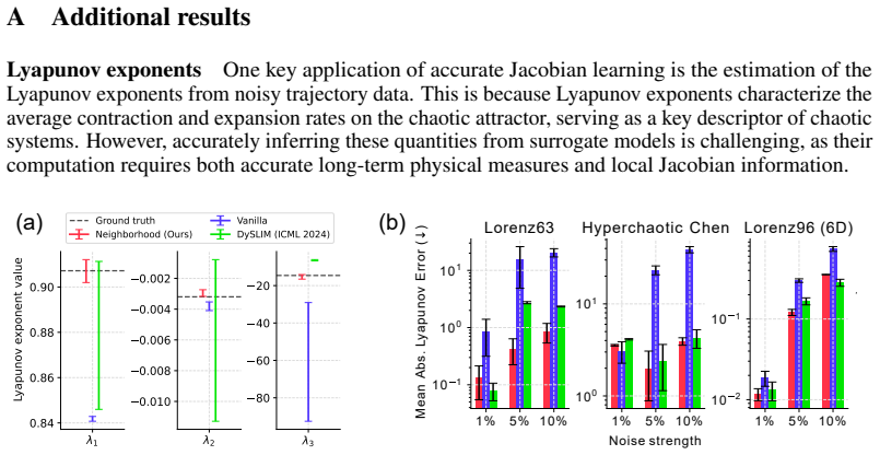
C. Ziehmann, L. A. Smith, and J. Kurths. Localized Lyapunov exponents and the prediction of predictability.Physics Letters A, 271(4):237–251, 2000. 13 A Additional results Lyapunov exponentsOne key application of accurate Jacobian learning is the estimation of the Lyapunov exponents from noisy trajectory data. This is because Lyapunov exponents characteri...

work page 2000
[59]

Samplem= 50random initial points on the attractor

work page
[60]

Estimate the characteristic time scaleτof the system, via the average frequency spectrum

work page
[61]

Simulatemon-attractor trajectories in the time span[0,10τ]with∆t= 0.01τ

work page
[62]

x y z # =

Shift and scale datasets using the train dataset statistics. Sampling on-attractor initial pointsTo sample points on the chaotic attractor, we first drew m initial conditions{u i 0}m i=1 from a normal distribution, with the mean and standard deviation chosen so that the sampled points would lie in the basin of attraction of the chaotic attractor. Afterwar...

work page