pith. machine review for the scientific record. sign in

arxiv: 2605.14493 · v1 · submitted 2026-05-14 · 💰 econ.GN · q-fin.EC

Recognition: no theorem link

Deep Learning for Solving and Estimating Dynamic Models in Economics and Finance

Authors on Pith no claims yet

Pith reviewed 2026-05-15 01:25 UTC · model grok-4.3

classification 💰 econ.GN q-fin.EC
keywords deep learningdynamic stochastic modelscurse of dimensionalityeconomicsfinanceneural networksheterogeneous agentsvalue function iteration
0
0 comments X

The pith

Deep learning methods solve and estimate high-dimensional dynamic stochastic models in economics and finance by embedding equilibrium conditions into neural-network training.

A machine-rendered reading of the paper's core claim, the machinery that carries it, and where it could break.

The paper presents an implementation-focused overview of deep learning techniques to address the curse of dimensionality in dynamic economic models. It covers four main approaches: Deep Equilibrium Nets that incorporate discrete-time equilibrium conditions into loss functions, Physics-Informed Neural Networks that approximate continuous-time differential equations, deep surrogate models for fast differentiable approximations, and Gaussian-process methods that add uncertainty quantification to dynamic programming. These tools are illustrated on representative-agent models, heterogeneous-agent economies, overlapping-generations settings, macro-finance problems, and climate-economy applications, with code examples provided for direct experimentation.

Core claim

The central claim is that deep learning methods such as Deep Equilibrium Nets, Physics-Informed Neural Networks, deep surrogate models, and Gaussian-process dynamic programming can solve and estimate high-dimensional dynamic stochastic models in economics and finance that strain classical tensor-product grid methods.

What carries the argument

Deep Equilibrium Nets and Physics-Informed Neural Networks, which embed the model's equilibrium conditions or partial differential equations directly into the neural-network loss function to train approximations to policy and value functions.

If this is right

  • High-dimensional heterogeneous-agent and overlapping-generations models with aggregate risk become routinely solvable.
  • Structural estimation by simulated method of moments extends to economies with many state variables and frictions.
  • Continuous-time macro-finance models with occasionally binding constraints can be solved without discretization grids.
  • Climate-economy models under uncertainty support sensitivity analysis and policy design with quantified approximation error.
  • Gaussian-process dynamic programming combined with active learning scales value-function iteration to very large continuous state spaces.

Where Pith is reading between the lines

These are editorial extensions of the paper, not claims the author makes directly.

  • If the methods remain stable at scale, they could support real-time policy evaluation in models previously considered computationally prohibitive.
  • The surrogate-model and uncertainty-quantification components may enable tighter integration between structural estimation and machine-learning forecasting pipelines.
  • Active-learning variants could reduce the number of model evaluations needed for accurate solutions in high-dimensional spaces.

Load-bearing premise

The neural-network approximations remain accurate and stable when applied to the equilibrium conditions and dynamics of the high-dimensional models without introducing material bias or convergence failures.

What would settle it

A direct numerical comparison in which the deep-learning solutions produce policy functions or equilibrium prices that deviate materially from known analytical solutions or converged low-dimensional grid benchmarks on a specific high-dimensional test case.

Figures

Figures reproduced from arXiv: 2605.14493 by Simon Scheidegger.

Figure 1.1
Figure 1.1. Figure 1.1: The three enablers of the deep-learning revolution: large-scale data, massively parallel [PITH_FULL_IMAGE:figures/full_fig_p021_1_1.png] view at source ↗
Figure 1.2
Figure 1.2. Figure 1.2: Supervised learning: regression. The model [PITH_FULL_IMAGE:figures/full_fig_p022_1_2.png] view at source ↗
Figure 1.3
Figure 1.3. Figure 1.3: Supervised learning: classification. A linear decision boundary separates low-risk [PITH_FULL_IMAGE:figures/full_fig_p023_1_3.png] view at source ↗
Figure 1.4
Figure 1.4. Figure 1.4: Unsupervised learning: clustering. Unlabeled data points are grouped into three [PITH_FULL_IMAGE:figures/full_fig_p023_1_4.png] view at source ↗
Figure 1.5
Figure 1.5. Figure 1.5: Reinforcement learning: the agent–environment loop. The agent observes a state, [PITH_FULL_IMAGE:figures/full_fig_p024_1_5.png] view at source ↗
Figure 1.6
Figure 1.6. Figure 1.6: The three-step supervised-learning recipe that underpins every model in this course. [PITH_FULL_IMAGE:figures/full_fig_p025_1_6.png] view at source ↗
Figure 1.7
Figure 1.7. Figure 1.7: Binary classification with a sigmoid output. A scalar score [PITH_FULL_IMAGE:figures/full_fig_p026_1_7.png] view at source ↗
Figure 1.8
Figure 1.8. Figure 1.8: Binary cross-entropy and mean squared error as functions of the predicted class [PITH_FULL_IMAGE:figures/full_fig_p026_1_8.png] view at source ↗
Figure 1.9
Figure 1.9. Figure 1.9: An artificial neuron in the McCulloch–Pitts lineage. Inputs [PITH_FULL_IMAGE:figures/full_fig_p028_1_9.png] view at source ↗
Figure 1.10
Figure 1.10. Figure 1.10: An L-layer deep feedforward network. Each layer applies an affine map followed by a pointwise nonlinearity; the composition realizes Eq. (1.6). Depth (rather than width) is what gives neural networks their efficient representational power for compositionally structured functions. classes forming concentric spirals); each hidden layer warps the space so that the data become progressively more linearly se… view at source ↗
Figure 1.11
Figure 1.11. Figure 1.11: Schematic loss-trajectory comparison on a moderately ill-conditioned objective. [PITH_FULL_IMAGE:figures/full_fig_p032_1_11.png] view at source ↗
Figure 1.12
Figure 1.12. Figure 1.12: Three common learning-rate schedules. A constant rate is simple but often converges [PITH_FULL_IMAGE:figures/full_fig_p032_1_12.png] view at source ↗
Figure 1.13
Figure 1.13. Figure 1.13: Backpropagation as forward and backward passes through the network. The [PITH_FULL_IMAGE:figures/full_fig_p033_1_13.png] view at source ↗
Figure 1.14
Figure 1.14. Figure 1.14: Seven representative activation functions from Table [PITH_FULL_IMAGE:figures/full_fig_p035_1_14.png] view at source ↗
Figure 1.15
Figure 1.15. Figure 1.15: Distribution of pre-activations at one hidden neuron, sampled at three points [PITH_FULL_IMAGE:figures/full_fig_p037_1_15.png] view at source ↗
Figure 1.16
Figure 1.16. Figure 1.16: Schematic of the double-descent phenomenon. In the classical regime ( [PITH_FULL_IMAGE:figures/full_fig_p040_1_16.png] view at source ↗
Figure 1.17
Figure 1.17. Figure 1.17: An unrolled Recurrent Neural Network. The same parameters [PITH_FULL_IMAGE:figures/full_fig_p042_1_17.png] view at source ↗
Figure 1.18
Figure 1.18. Figure 1.18: The LSTM cell. The green top lane is the [PITH_FULL_IMAGE:figures/full_fig_p043_1_18.png] view at source ↗
Figure 1.19
Figure 1.19. Figure 1.19: renders the attention pattern of the worked “cat/it” example on a compressed five-token version of the sentence. The output oit is the new representation at the “it” position, formed as a weighted average of the values, with most weight coming from “cat”. the cat sat mat it 0.05 0.58 0.08 0.20 0.09 qit oit keys and values at each token position How to read the arrows 1. Blue down arrow: build the query … view at source ↗
Figure 1.20
Figure 1.20. Figure 1.20: One Transformer block in pre-norm form. Self-attention first mixes information across token positions, then the pointwise MLP transforms each token separately. The red skip paths are the residual connections that let deep stacks train stably. A full Transformer stacks L such blocks; GPT-3, for instance, uses L = 96. the theoretical peak throughput. This is why modern foundation models, GPT-n, BERT, ViT,… view at source ↗
Figure 2.1
Figure 2.1. Figure 2.1: The volume paradox behind the curse of dimensionality. [PITH_FULL_IMAGE:figures/full_fig_p055_2_1.png] view at source ↗
Figure 2.2
Figure 2.2. Figure 2.2: Grid-based vs. simulation-based state sampling. A Cartesian grid (left) allocates effort [PITH_FULL_IMAGE:figures/full_fig_p056_2_2.png] view at source ↗
Figure 2.3
Figure 2.3. Figure 2.3: Why a “random” point in high dimensions lives on the shell, not in the core. [PITH_FULL_IMAGE:figures/full_fig_p057_2_3.png] view at source ↗
Figure 2.4
Figure 2.4. Figure 2.4: Supervised learning (left) versus DEQN training (right). Both paradigms train a [PITH_FULL_IMAGE:figures/full_fig_p058_2_4.png] view at source ↗
Figure 2.5
Figure 2.5. Figure 2.5: Schematic, not measured: the qualitative convergence behavior typical of a successful [PITH_FULL_IMAGE:figures/full_fig_p061_2_5.png] view at source ↗
Figure 2.6
Figure 2.6. Figure 2.6: Hard vs. soft constraints in the DEQN architecture for Brock–Mirman. The network [PITH_FULL_IMAGE:figures/full_fig_p063_2_6.png] view at source ↗
Figure 2.7
Figure 2.7. Figure 2.7: Two paradigms for numerical integration that underlie every rule in this section. [PITH_FULL_IMAGE:figures/full_fig_p065_2_7.png] view at source ↗
Figure 2.8
Figure 2.8. Figure 2.8: Geometric meaning of a central finite difference. The derivative [PITH_FULL_IMAGE:figures/full_fig_p069_2_8.png] view at source ↗
Figure 2.9
Figure 2.9. Figure 2.9: The classic U-curve of central finite differences, here for [PITH_FULL_IMAGE:figures/full_fig_p070_2_9.png] view at source ↗
Figure 2.10
Figure 2.10. Figure 2.10: The two modes of autodiff on y = x 2 + sin(x) at x = 2. Top: forward mode carries a derivative tag v˙ = ∂v/∂x alongside each value and reads y˙ = dy/dx at the output. Bottom: reverse mode evaluates f forward, stores the graph, then walks backwards with v¯ = ∂y/∂v and reads x¯ = dy/dx at the input. Both deliver 3.584, equal to f ′ (2) = 2 · 2 + cos(2) at machine precision. Forward mode scales linearly wi… view at source ↗
Figure 2.11
Figure 2.11. Figure 2.11: Convergence of the relative Euler-error distribution under six different loss kernels on [PITH_FULL_IMAGE:figures/full_fig_p076_2_11.png] view at source ↗
Figure 3.1
Figure 3.1. Figure 3.1: The Fischer–Burmeister complementarity function, drawn in the investment–multiplier [PITH_FULL_IMAGE:figures/full_fig_p087_3_1.png] view at source ↗
Figure 3.2
Figure 3.2. Figure 3.2: Quadrature-cost crossover for the IRBC model as a function of the number of countries [PITH_FULL_IMAGE:figures/full_fig_p089_3_2.png] view at source ↗
Figure 3.3
Figure 3.3. Figure 3.3: Reference network architecture used for the [PITH_FULL_IMAGE:figures/full_fig_p090_3_3.png] view at source ↗
Figure 4.1
Figure 4.1. Figure 4.1: Why random search beats grid search when only one hyperparameter matters. Both [PITH_FULL_IMAGE:figures/full_fig_p099_4_1.png] view at source ↗
Figure 4.2
Figure 4.2. Figure 4.2: Bayesian optimization in one dimension. All curves come from a genuine Gaussian [PITH_FULL_IMAGE:figures/full_fig_p100_4_2.png] view at source ↗
Figure 4.3
Figure 4.3. Figure 4.3: Successive Halving with 81 initial candidates and reduction factor [PITH_FULL_IMAGE:figures/full_fig_p101_4_3.png] view at source ↗
Figure 4.4
Figure 4.4. Figure 4.4: Stylized sketch of the multi-component loss-scale problem, drawn to mimic what one typically sees early in a two-country IRBC training run; this is not measured data. The three curves are hand-picked exponentials ak e −t/τk (with a1=50, τ1=150; a2=0.5, τ2=750; a3=5, τ3=200), chosen only to make the mechanism visible: at initialization the residuals differ by about two orders of magnitude, and under unifo… view at source ↗
Figure 5.1
Figure 5.1. Figure 5.1: Stylized lifecycle profiles in an OLG economy (schematic, [PITH_FULL_IMAGE:figures/full_fig_p110_5_1.png] view at source ↗
Figure 5.2
Figure 5.2. Figure 5.2: Closed-form savings rates βh from [PITH_FULL_IMAGE:figures/full_fig_p113_5_2.png] view at source ↗
Figure 6.1
Figure 6.1. Figure 6.1: Genealogy of the heterogeneous-agent models treated in this script. This chapter [PITH_FULL_IMAGE:figures/full_fig_p125_6_1.png] view at source ↗
Figure 6.2
Figure 6.2. Figure 6.2: Linear interpolation in Young’s method. Mass [PITH_FULL_IMAGE:figures/full_fig_p128_6_2.png] view at source ↗
Figure 6.3
Figure 6.3. Figure 6.3: Young’s cascade for one source bin (essentially Fig. 1 of [PITH_FULL_IMAGE:figures/full_fig_p130_6_3.png] view at source ↗
Figure 6.4
Figure 6.4. Figure 6.4: Flow diagram for one forward step of Young’s histogram update (Algorithm [PITH_FULL_IMAGE:figures/full_fig_p133_6_4.png] view at source ↗
Figure 6.5
Figure 6.5. Figure 6.5: Young’s histogram (left) versus Monte Carlo panel simulation (right). Both approxi [PITH_FULL_IMAGE:figures/full_fig_p133_6_5.png] view at source ↗
Figure 6.6
Figure 6.6. Figure 6.6: Histogram encoding and neural network architecture. The individual state [PITH_FULL_IMAGE:figures/full_fig_p135_6_6.png] view at source ↗
Figure 6.7
Figure 6.7. Figure 6.7: Two ways to encode the aggregate state in deep equilibrium learning. Each pipeline [PITH_FULL_IMAGE:figures/full_fig_p142_6_7.png] view at source ↗
Figure 6.8
Figure 6.8. Figure 6.8: Intuition for sequence space in Brock–Mirman. [PITH_FULL_IMAGE:figures/full_fig_p144_6_8.png] view at source ↗
Figure 6.9
Figure 6.9. Figure 6.9: Training flow for sequence-space DEQNs. The exogenous shock history is the network [PITH_FULL_IMAGE:figures/full_fig_p145_6_9.png] view at source ↗
Figure 7.1
Figure 7.1. Figure 7.1: Discrete-time DEQNs and continuous-time PINNs use the same residual-minimization [PITH_FULL_IMAGE:figures/full_fig_p155_7_1.png] view at source ↗
Figure 7.2
Figure 7.2. Figure 7.2: PINN solution of the 1D ODE y ′′ = −1 on (0, 1) with y(0) = y(1) = 0 and the soft￾penalty loss (7.4). The analytical solution 1 2 x(1 − x) (solid blue) is recovered to plotting accuracy by the converged network (dotted green); the dashed red curve illustrates a typical early-training iterate, which still misses the endpoints because the boundary penalty is enforced only approxi￾mately. Tick marks on the … view at source ↗
Figure 7.3
Figure 7.3. Figure 7.3: Failure modes of soft boundary-condition enforcement on a Dirichlet problem with [PITH_FULL_IMAGE:figures/full_fig_p158_7_3.png] view at source ↗
Figure 7.4
Figure 7.4. Figure 7.4: Hard boundary-condition decomposition for the trial solution [PITH_FULL_IMAGE:figures/full_fig_p158_7_4.png] view at source ↗
Figure 7.5
Figure 7.5. Figure 7.5: PINN solution of the 1D ODE y ′′ + y = 0 on [0, π/2] with the hard-BC trial solution (7.6). The analytical solution sin(x) (solid blue) is recovered to plotting accuracy by the converged network (dotted green); the dashed red curve illustrates a typical early-training iterate. Tick marks on the x-axis are the uniformly drawn collocation points. The curves above are TikZ illustrations rather than direct e… view at source ↗
Figure 7.6
Figure 7.6. Figure 7.6: The DGM (Deep Galerkin Method) architecture of [PITH_FULL_IMAGE:figures/full_fig_p163_7_6.png] view at source ↗
Figure 7.7
Figure 7.7. Figure 7.7: Operator learning generalizes PINNs by amortising over an entire parametric family of [PITH_FULL_IMAGE:figures/full_fig_p169_7_7.png] view at source ↗
Figure 8.1
Figure 8.1. Figure 8.1: Three simulated standard Brownian sample paths [PITH_FULL_IMAGE:figures/full_fig_p174_8_1.png] view at source ↗
Figure 8.2
Figure 8.2. Figure 8.2: Stationary continuous-time heterogeneous-agent equilibrium as a coupled HJB–KFE– [PITH_FULL_IMAGE:figures/full_fig_p179_8_2.png] view at source ↗
Figure 8.3
Figure 8.3. Figure 8.3: Stationary cross-sectional densities g ∗ in the two benchmarks, by productivity type n ∈ {n1, n2} (low and high). In both economies, only the constrained low-productivity type n1 supports a Dirac atom at the borrowing constraint (blue spike): high-productivity households are not bound. Left: Huggett, bonds with limit b = −2 and zero net supply, so the bulk of mass sits around b = 0. Right: Aiyagari, capi… view at source ↗
Figure 9.1
Figure 9.1. Figure 9.1: Why surrogates help. Left: structural estimation, uncertainty quantification, and optimal policy design are outer loops over a parameter vector θ, and the direct implementation re-solves the full model inside the loop, so the cost scales with the number of outer iterations times the per-solve cost. Right: a surrogate moves that solve into a one-time offline phase, solving the model only at a design of ex… view at source ↗
Figure 9.2
Figure 9.2. Figure 9.2: Pseudo-state surrogate architecture. Economic states [PITH_FULL_IMAGE:figures/full_fig_p192_9_2.png] view at source ↗
Figure 9.3
Figure 9.3. Figure 9.3: Squared-exponential kernel as a function of distance for three length scales. Small [PITH_FULL_IMAGE:figures/full_fig_p194_9_3.png] view at source ↗
Figure 9.4
Figure 9.4. Figure 9.4: Gaussian-process prior and posterior on a 1D regression problem. [PITH_FULL_IMAGE:figures/full_fig_p195_9_4.png] view at source ↗
Figure 9.5
Figure 9.5. Figure 9.5: Marginal-likelihood Occam’s razor for a GP. As the kernel becomes more flexible [PITH_FULL_IMAGE:figures/full_fig_p196_9_5.png] view at source ↗
Figure 9.6
Figure 9.6. Figure 9.6: Bayesian Active Learning in action. (a) Starting from three initial observations (red dots), the GP posterior mean (blue line) deviates from the true function (dashed black) in the data-sparse region, where the 95% credible band (blue shading) is wide. (b) The acquisition function selects the point of maximum posterior variance (green diamond); after evaluation, the posterior tightens locally and the mea… view at source ↗
Figure 9.7
Figure 9.7. Figure 9.7: Inducing-point intuition. Exact GP inference conditions on all [PITH_FULL_IMAGE:figures/full_fig_p200_9_7.png] view at source ↗
Figure 9.8
Figure 9.8. Figure 9.8: Spectral decay of the active-subspace eigenvalues for a schematic example with [PITH_FULL_IMAGE:figures/full_fig_p202_9_8.png] view at source ↗
Figure 9.9
Figure 9.9. Figure 9.9: Linear active-subspace pipeline. Gradient samples identify the dominant eigenspace of [PITH_FULL_IMAGE:figures/full_fig_p203_9_9.png] view at source ↗
Figure 9.10
Figure 9.10. Figure 9.10: Stylized comparison of the two selection criteria for the radial-ridge target [PITH_FULL_IMAGE:figures/full_fig_p205_9_10.png] view at source ↗
Figure 9.11
Figure 9.11. Figure 9.11: Deep active-subspace pipeline. Input–output pairs [PITH_FULL_IMAGE:figures/full_fig_p205_9_11.png] view at source ↗
Figure 9.12
Figure 9.12. Figure 9.12: Same-budget active enrichment inside one-dimensional GP value-function iteration. [PITH_FULL_IMAGE:figures/full_fig_p211_9_12.png] view at source ↗
Figure 10.1
Figure 10.1. Figure 10.1: The two-layer surrogate architecture for surrogate-based SMM, read top-to-bottom [PITH_FULL_IMAGE:figures/full_fig_p225_10_1.png] view at source ↗
Figure 10.2
Figure 10.2. Figure 10.2: Direct SMM criterion for the joint Brock–Mirman estimation. The left panel uses [PITH_FULL_IMAGE:figures/full_fig_p227_10_2.png] view at source ↗
Figure 11.1
Figure 11.1. Figure 11.1: The integrated-assessment feedback loop. The economy produces output and CO [PITH_FULL_IMAGE:figures/full_fig_p231_11_1.png] view at source ↗
Figure 11.2
Figure 11.2. Figure 11.2: Business-as-usual industrial emissions in CDICE (in GtCO [PITH_FULL_IMAGE:figures/full_fig_p236_11_2.png] view at source ↗
Figure 11.3
Figure 11.3. Figure 11.3: Topology of the CDICE climate side. Total emissions [PITH_FULL_IMAGE:figures/full_fig_p237_11_3.png] view at source ↗
Figure 11.4
Figure 11.4. Figure 11.4: Atmospheric carbon MAT t along the BAU path (in GtC, over 200 years from 2015) under the three CDICE carbon-cycle calibrations (CDICE = MMM, CDICE-MESMO, CDICE-LOVECLIM) and the legacy DICE-2016 carbon cycle. Only the carbon-cycle block is varied here; the temperature block is held at the CDICE MMM calibration, since the BAU carbon-stock path does not depend on the temperature calibration to first order… view at source ↗
Figure 11.5
Figure 11.5. Figure 11.5: Schematic of the two qualitative features reported by [PITH_FULL_IMAGE:figures/full_fig_p251_11_5.png] view at source ↗
Figure 11.6
Figure 11.6. Figure 11.6: Schematic of the total-effect Sobol shares of [PITH_FULL_IMAGE:figures/full_fig_p254_11_6.png] view at source ↗
Figure 11.7
Figure 11.7. Figure 11.7: Climate side of CDICE versus TCRE. The 5-state CDICE module on the left, in [PITH_FULL_IMAGE:figures/full_fig_p256_11_7.png] view at source ↗
Figure 11.8
Figure 11.8. Figure 11.8: Business-as-usual baseline for the 12-cohort stochastic OLG-IAM of [PITH_FULL_IMAGE:figures/full_fig_p257_11_8.png] view at source ↗
Figure 11.9
Figure 11.9. Figure 11.9: Three-step machine-learning pipeline for constrained carbon-tax design. The DEQN [PITH_FULL_IMAGE:figures/full_fig_p257_11_9.png] view at source ↗
Figure 11.10
Figure 11.10. Figure 11.10: Gaussian-process welfare surrogate over the two-dimensional tax-parameter slice [PITH_FULL_IMAGE:figures/full_fig_p258_11_10.png] view at source ↗
Figure 11.11
Figure 11.11. Figure 11.11: Welfare-improving but not Pareto-improving cumulative-emissions tax with a fixed [PITH_FULL_IMAGE:figures/full_fig_p260_11_11.png] view at source ↗
Figure 11.12
Figure 11.12. Figure 11.12: Pareto-improving cumulative-emissions tax with optimized intergenerational [PITH_FULL_IMAGE:figures/full_fig_p262_11_12.png] view at source ↗
Figure 11.13
Figure 11.13. Figure 11.13: Optimized transfer-share profile ωj across the 12 cohorts alive at t = 0, drawn directly from (11.59). The profile is decidedly non-monotone: the largest shares go to cohorts 1 (oldest), 5, and 8, which are precisely the cohorts the participation constraint U˜ t ≥ Ut binds most tightly for under the un-transferred tax of [PITH_FULL_IMAGE:figures/full_fig_p263_11_13.png] view at source ↗
Figure 12.1
Figure 12.1. Figure 12.1: The shared computational workflow of the four methods of this course (DEQNs, [PITH_FULL_IMAGE:figures/full_fig_p269_12_1.png] view at source ↗
Figure 12.2
Figure 12.2. Figure 12.2: Bridges between the four method families. The core box restates the shared workflow: [PITH_FULL_IMAGE:figures/full_fig_p272_12_2.png] view at source ↗
read the original abstract

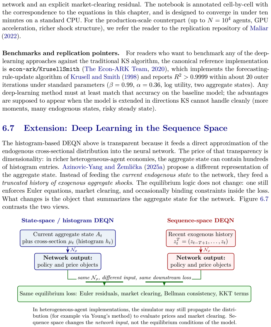
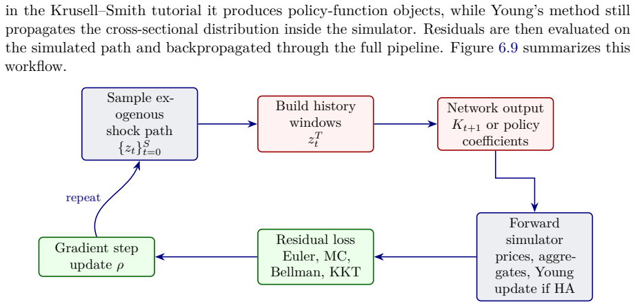
This script offers an implementation-oriented introduction to deep learning methods for solving and estimating high-dimensional dynamic stochastic models in economics and finance. Its starting point is the curse of dimensionality: heterogeneous-agent economies, overlapping-generations models with aggregate risk, continuous-time models with occasionally binding constraints, climate-economy models, and macro-finance environments with many assets and frictions generate state and parameter spaces that strain classical tensor-product grid methods. The exposition is organized around four complementary methodologies. Deep Equilibrium Nets embed discrete-time equilibrium conditions into neural-network loss functions. Physics-Informed Neural Networks approximate continuous-time Hamilton--Jacobi--Bellman, Kolmogorov forward, and related partial differential equations. Deep surrogate models provide fast, differentiable approximations to expensive structural models, while Gaussian processes add a probabilistic layer that quantifies approximation uncertainty; together they support estimation, sensitivity analysis, and constrained policy design. Gaussian-process-based dynamic programming, combined with active learning and dimension reduction, extends value-function iteration to very large continuous state spaces. Applications span representative-agent and international real business cycle models, overlapping-generations and heterogeneous-agent economies, continuous-time macro-finance, structural estimation by simulated method of moments, and climate economics under uncertainty. Companion notebooks in TensorFlow and PyTorch invite hands-on experimentation. These notes are a deliberately subjective and inevitably incomplete snapshot of a rapidly evolving field, aimed at equipping PhD students and researchers to engage with this frontier hands-on.

Editorial analysis

A structured set of objections, weighed in public.

Desk editor's note, referee report, simulated authors' rebuttal, and a circularity audit. Tearing a paper down is the easy half of reading it; the pith above is the substance, this is the friction.

Referee Report

1 major / 3 minor

Summary. The manuscript is an implementation-oriented tutorial introducing four deep-learning approaches—Deep Equilibrium Nets, Physics-Informed Neural Networks, deep surrogate models, and Gaussian-process dynamic programming—for solving and estimating high-dimensional dynamic stochastic models in economics and finance. It frames these methods as practical responses to the curse of dimensionality in heterogeneous-agent, overlapping-generations, continuous-time macro-finance, and climate-economy settings, supplies companion TensorFlow/PyTorch notebooks, and positions the notes as a subjective snapshot of the literature aimed at PhD students and researchers.

Significance. If the neural-network approximations remain accurate and stable for the equilibrium conditions and dynamics described, the paper would be significant as a hands-on bridge between classical solution techniques and scalable deep-learning tools, enabling faster iteration on otherwise intractable models and supporting estimation, sensitivity analysis, and policy design in macro-finance and climate economics.

major comments (1)
  1. [methodologies overview and applications] The central claim that the four methodologies can reliably address models that strain tensor-product grids rests on the accuracy and stability of the neural approximations; the manuscript treats these properties as established by the cited literature without providing new error bounds, convergence diagnostics, or side-by-side benchmarks against classical methods within the text itself.
minor comments (3)
  1. [abstract] The abstract states that the notes are 'deliberately subjective and inevitably incomplete'; a short explicit statement of scope limitations (e.g., which model classes are omitted) would help readers calibrate expectations.
  2. [throughout] Notation for state variables, value functions, and equilibrium conditions is introduced separately for each methodology; a brief consolidated table or appendix would improve cross-section readability.
  3. [Gaussian-process dynamic programming] The description of Gaussian-process dynamic programming mentions active learning and dimension reduction but does not specify the exact acquisition function or reduction technique used in the accompanying notebook.

Simulated Author's Rebuttal

1 responses · 0 unresolved

We thank the referee for the positive evaluation and the recommendation of minor revision. We address the single major comment below.

read point-by-point responses
  1. Referee: The central claim that the four methodologies can reliably address models that strain tensor-product grids rests on the accuracy and stability of the neural approximations; the manuscript treats these properties as established by the cited literature without providing new error bounds, convergence diagnostics, or side-by-side benchmarks against classical methods within the text itself.

    Authors: We agree that the manuscript relies on accuracy and stability results established in the cited literature rather than deriving new error bounds or conducting original side-by-side benchmarks. This is consistent with the paper's stated scope as an implementation-oriented tutorial and subjective snapshot of the literature, whose goal is to equip readers to apply the methods and consult the original sources for theoretical details. To address the concern, we will add a concise new subsection titled 'Accuracy, Stability, and Practical Diagnostics' that summarizes key convergence guarantees and numerical validation practices from the referenced works (e.g., those on Deep Equilibrium Nets and PINNs). We will also insert brief pointers to existing benchmark studies in the applications sections and note in the introduction that users should perform model-specific verification. These changes preserve the tutorial focus while making the reliance on prior results more transparent. revision: partial

Circularity Check

0 steps flagged

No significant circularity

full rationale

The paper is an implementation-oriented tutorial and review that organizes four families of existing deep-learning methods (Deep Equilibrium Nets, PINNs, deep surrogates, Gaussian-process dynamic programming) for high-dimensional economic models. It does not advance new derivations, uniqueness theorems, or fitted parameters whose outputs are then relabeled as predictions within the manuscript itself. All central claims rest on summaries of prior literature plus external notebooks for verification; no equation or step reduces by construction to a self-defined input or self-citation chain. The accuracy and stability of the approximations are treated as established properties of the cited techniques rather than results derived inside this document.

Axiom & Free-Parameter Ledger

0 free parameters · 1 axioms · 0 invented entities

The paper relies on standard assumptions from dynamic stochastic general equilibrium theory and prior deep-learning literature; no new free parameters, axioms, or invented entities are introduced in the abstract.

axioms (1)
  • domain assumption Standard dynamic stochastic general equilibrium assumptions hold for the models discussed.
    The methods are presented as applicable to representative-agent, heterogeneous-agent, and continuous-time models common in the field.

pith-pipeline@v0.9.0 · 5546 in / 1187 out tokens · 69870 ms · 2026-05-15T01:25:56.737540+00:00 · methodology

discussion (0)

Sign in with ORCID, Apple, or X to comment. Anyone can read and Pith papers without signing in.

Reference graph

Works this paper leans on

13 extracted references · 13 canonical work pages · 4 internal anchors

  1. [1]

    Achdou, Y., Han, J., Lasry, J.-M., Lions, P.-L., and Moll, B. (2022). Income and wealth distribution in macroeconomics: A continuous-time approach.The Review of Economic Studies, 89(1):45–86. Adjemian, S., Bastani, H., Juillard, M., Karamé, F., Maih, J., Mihoubi, F., Mutschler, W., Pfeifer, J., Ratto, M., Rion, N., and Villemot, S. (2024). Dynare: Referen...

  2. [2]

    Solving Nonlinear and High-Dimensional Partial Differential Equations via Deep Learning

    Dynare Working Papers 80, CEPREMAP. Aggarwal, C. C., Hinneburg, A., and Keim, D. A. (2001). On the surprising behavior of distance metrics in high dimensional space. InDatabase Theory — ICDT 2001, volume 1973 ofLecture Notes in Computer Science, pages 420–434. Springer. Aiyagari, S. R. (1994). Uninsured idiosyncratic risk and aggregate saving.The Quarterl...

  3. [3]

    and Luetticke, R

    Bayer, C. and Luetticke, R. (2020). Solving discrete time heterogeneous agent models with aggre- gate risk and many idiosyncratic states by perturbation.Quantitative Economics, 11(4):1253–

  4. [4]

    Belkin, M., Hsu, D., Ma, S., and Mandal, S. (2019). Reconciling modern machine-learning practice and the classical bias–variance trade-off.Proceedings of the National Academy of Sciences, 116(32):15849–15854. Bellman, R. (1957).Dynamic Programming. Princeton University Press, Princeton, NJ. Bellman, R. (1961).Adaptive Control Processes: A Guided Tour. ’Ra...

  5. [5]

    P., Faisal, A

    Deisenroth, M. P., Faisal, A. A., and Ong, C. S. (2020).Mathematics for Machine Learning. Cambridge University Press, Cambridge. Deisenroth, M. P. and Rasmussen, C. E. (2011). PILCO: A model-based and data-efficient approach to policy search. InProceedings of the 28th International Conference on Machine Learning. Deisenroth, M. P., Rasmussen, C. E., and P...

  6. [6]

    Non-stochasticbestarmidentificationandhyperparameter optimization

    Jamieson, K.andTalwalkar, A.(2016). Non-stochasticbestarmidentificationandhyperparameter optimization. InProceedings of the 19th International Conference on Artificial Intelligence and Statistics (AISTATS). Jensen, S. and Traeger, C. P. (2014). Optimal climate change mitigation under long-term growth uncertainty: Stochastic integrated assessment and analy...

  7. [7]

    Scaling Laws for Neural Language Models

    Kahou, M. E., Fernández-Villaverde, J., Perla, J., and Sood, A. (2021). Exploiting symmetry in high-dimensional dynamic programming. NBER Working Paper 28981, National Bureau of Economic Research. Kaplan, G., Moll, B., and Violante, G. L. (2018). Monetary policy according to HANK.American Economic Review, 108(3):697–743. Kaplan, J., McCandlish, S., Henigh...

  8. [8]

    and Lions, P.-L

    Lasry, J.-M. and Lions, P.-L. (2007). Mean field games.Japanese Journal of Mathematics, 2(1):229–260. Leach, A. J. (2007). The climate change learning curve.Journal of Economic Dynamics and Control, 31(5):1728–1752. LeCun, Y., Bengio, Y., and Hinton, G. (2015). Deep learning.Nature, 521(7553):436–444. 321 Lee, B.-S. and Ingram, B. F. (1991). Simulation es...

  9. [9]

    arXiv:1908.08681 , author =

    Elsevier. Maliar, L., Maliar, S., and Valli, F. (2010). Solving the incomplete markets model with aggregate uncertainty using the Krusell–Smith algorithm.Journal of Economic Dynamics and Control, 34(1):42–49. Maliar, L., Maliar, S., and Winant, P. (2021). Deep learning for solving dynamic economic models.Journal of Monetary Economics, 122:76–101. Maliar, ...

  10. [10]

    Nordhaus, W. D. and Yang, Z. (1996). A regional dynamic general-equilibrium model of alternative climate-change strategies.The American Economic Review, pages 741–765. Norets, A. (2012). Estimation of dynamic discrete choice models using artificial neural network approximations.Econometric Reviews, 31(1):84–106. Novak, E. and Woźniakowski, H. (2008).Tract...

  11. [11]

    and D’Hombres, B

    Saltelli, A. and D’Hombres, B. (2010). Sensitivity analysis didn’t help. A practitioner’s critique of the Stern review.Global Environmental Change, 20(2):298–302. Saltelli, A., Ratto, M., Andres, T., Campolongo, F., Cariboni, J., Gatelli, D., Saisana, M., and Tarantola, S. (2008).Global Sensitivity Analysis: The Primer. Wiley. Santurkar, S., Tsipras, D., ...

  12. [12]

    324 Sargent, T. J. and Stachurski, J. (2026). Dynamic programming, volumes i and ii. QuantEcon open textbook series. Scheidegger, S. and Bilionis, I. (2019). Machine learning for high-dimensional dynamic stochastic economies.Journal of Computational Science, 33:68 –

  13. [13]

    Horovod: fast and easy distributed deep learning in TensorFlow

    Scheidegger, S. and Treccani, A. (2018). Pricing american options under high-dimensional models with recursive adaptive sparse expectations.Journal of Financial Econometrics. Schlag, I., Irie, K., and Schmidhuber, J. (2021). Linear transformers are secretly fast weight programmers. InProceedings of the 38th International Conference on Machine Learning (IC...