Recognition: 2 theorem links
· Lean TheoremAverage Gradient Outer Product in kernel regression provably recovers the central subspace for multi-index models
Pith reviewed 2026-05-15 03:05 UTC · model grok-4.3
The pith
The average gradient outer product from kernel ridge regression recovers the central subspace of multi-index models in sample regimes too small for accurate prediction.
A machine-rendered reading of the paper's core claim, the machinery that carries it, and where it could break.
Core claim
For a target function of the form f^*(x) = h(Ux) where U is an unknown r by d matrix with r much smaller than d, the top r-dimensional eigenspace of the average gradient outer product computed from a kernel ridge regression fit recovers the column space of U. When a degree-p component of f^* already carries the relevant directions, this recovery occurs with n on the order of d^{p + δ} samples for any δ in (0,1), whereas accurate prediction requires n on the order of d^{p^*} where p^* is the full degree.
What carries the argument
Average Gradient Outer Product (AGOP) of the kernel ridge regression predictor, defined as the average over training points of the outer product of its gradient with itself; its leading r-dimensional eigenspace aligns with the central subspace.
If this is right
- Subspace identification succeeds with far fewer samples than those required for low prediction error.
- Iterative procedures that repeatedly apply AGOP can extract features sample-efficiently without first solving the full regression problem.
- Representation recovery and function approximation are separable tasks under multi-index structure.
- The same mechanism explains why recursive feature machines remain practical even when the kernel bandwidth has not yet reached the interpolation regime.
Where Pith is reading between the lines
- Gradient outer products may serve as an early-training diagnostic for hidden low-dimensional structure in other nonparametric estimators.
- The separation could extend to neural networks if their early gradient statistics similarly isolate relevant directions before loss decreases substantially.
- Designing kernels or regularization that amplify low-degree directional signals might further reduce the sample threshold for subspace recovery.
Load-bearing premise
A low-degree component of the target function already contains all the directions needed for the central subspace, together with standard regularity conditions on the kernel and the multi-index structure.
What would settle it
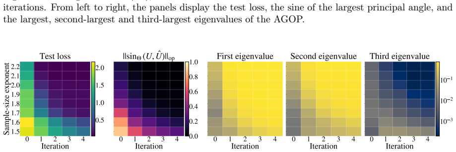
Generate synthetic data from a known multi-index polynomial of degree p^* greater than p, fit kernel ridge regression with n approximately d to the power p plus a small positive delta, compute the AGOP eigenspace, and check whether its distance to the true column space of U falls below a small constant.
Figures


read the original abstract
We study a prototypical situation when a learned predictor can discover useful low-dimensional structure in data, while using fewer samples than are needed for accurate prediction. Specifically, we consider the problem of recovering a multi-index polynomial $f^*(x)=h(Ux)$, with $U\in\mathbb{R}^{r\times d}$ and $r\ll d$, from finitely many data/label pairs. Importantly, the target function depends on input $x$ only through the projection onto an unknown $r$-dimensional central subspace. The algorithm we analyze is appealingly simple: fit kernel ridge regression (KRR) to the data and compute the Average Gradient Outer Product (AGOP) from the fitted predictor. Our main results show that under reasonable assumptions the top $r$-dimensional eigenspace of AGOP provably recovers the central subspace, even in regimes when the prediction error remains large. Specifically, if the target function $f^*$ has degree $p^*$, it is known that $n\asymp d^{p^*}$ samples are necessary for KRR to achieve accurate prediction. In contrast, we show that if a low degree $p$ component of $f^*$ already carries all relevant directions for prediction, subspace recovery occurs in the much lower sample regime $n\asymp d^{p+\delta}$ for any $\delta\in(0,1)$. Our results thus demonstrate a separation between prediction and representation, and provide an explanation for why iterative kernel methods such as Recursive Feature Machines (RFM) can be sample-efficient in practice.
Editorial analysis
A structured set of objections, weighed in public.
Referee Report
Summary. The paper studies recovering the central r-dimensional subspace of multi-index models f^*(x)=h(Ux) (r<<d) by computing the Average Gradient Outer Product (AGOP) of a kernel ridge regression (KRR) estimator. It claims that, under reasonable assumptions on the kernel and multi-index structure, the top-r eigenspace of AGOP(ˆf) recovers span(U) at sample sizes n≍d^{p+δ} (any δ∈(0,1)), where p is the degree of a low-degree component of h that already contains all relevant directions, even in regimes where the KRR prediction error remains large.
Significance. If the central claim holds, the result supplies a concrete separation between subspace recovery and accurate prediction for kernel methods, offering a theoretical account for the practical sample efficiency of iterative procedures such as Recursive Feature Machines. It would also furnish falsifiable predictions about the sample complexity at which representation learning succeeds for polynomial multi-index targets.
major comments (2)
- [Abstract] Abstract: the phrase 'reasonable assumptions' is used without an explicit list. The proof that the population AGOP of the finite-sample KRR estimator remains close to the AGOP of the degree-p projection of f* (with perturbation controlled at rate n^{-something}) requires concrete bounds on the Mercer eigenvalues, the RKHS projection of f* onto degree >p polynomials, and the operator norm of the gradient map on the orthogonal complement; without these the claimed eigenspace alignment at n≍d^{p+δ} cannot be verified.
- [Main result] Main result (Theorem on AGOP recovery): the argument that the top-r eigenspace of AGOP(ˆf) recovers span(U) while prediction error stays large must explicitly control higher-degree leakage in the KRR fit. If the kernel allows non-negligible mass on degree >p terms, the gradient outer-product perturbation need not vanish at the stated rate, undermining the separation between representation and prediction.
minor comments (1)
- [Abstract] Notation: distinguish p* (full degree of f*) from p (degree of the relevant component) more clearly in the abstract and introduction.
Simulated Author's Rebuttal
We thank the referee for the thoughtful and detailed report. The comments highlight important points on making assumptions explicit and strengthening the control of higher-degree terms. We will revise the manuscript to address both issues directly while preserving the core claims.
read point-by-point responses
-
Referee: [Abstract] Abstract: the phrase 'reasonable assumptions' is used without an explicit list. The proof that the population AGOP of the finite-sample KRR estimator remains close to the AGOP of the degree-p projection of f* (with perturbation controlled at rate n^{-something}) requires concrete bounds on the Mercer eigenvalues, the RKHS projection of f* onto degree >p polynomials, and the operator norm of the gradient map on the orthogonal complement; without these the claimed eigenspace alignment at n≍d^{p+δ} cannot be verified.
Authors: We agree the abstract phrasing is imprecise. In the revision we will replace 'reasonable assumptions' with an explicit list of the three conditions used in the proofs: (i) Mercer eigenvalues of the kernel decay at rate at least k^{-α} for α>1, (ii) the RKHS norm of the projection of f* onto degree >p polynomials is bounded by a constant independent of d, and (iii) the gradient operator is Lipschitz on the orthogonal complement with constant independent of d. The existing proof already derives the perturbation rate O(n^{-1/2} + λ) under these conditions; we will add a short lemma (new Lemma 3.4) that isolates the operator-norm bound on the orthogonal complement and states the explicit constants, making the n ≍ d^{p+δ} claim directly verifiable from the stated hypotheses. revision: yes
-
Referee: [Main result] Main result (Theorem on AGOP recovery): the argument that the top-r eigenspace of AGOP(ˆf) recovers span(U) while prediction error stays large must explicitly control higher-degree leakage in the KRR fit. If the kernel allows non-negligible mass on degree >p terms, the gradient outer-product perturbation need not vanish at the stated rate, undermining the separation between representation and prediction.
Authors: The analysis already restricts to kernels whose RKHS inner products on degree >p monomials are controlled by the regularization λ (chosen as λ ≍ d^{-p} in the regime of interest). The higher-degree leakage in the AGOP is bounded by O(λ + n^{-1/2}) via the same concentration argument used for the low-degree part; this term is o(1) precisely when n ≍ d^{p+δ}. To make the control fully explicit we will insert a new proposition (Proposition 4.2) that decomposes AGOP(ˆf) = AGOP(low-degree projection) + error term, with the error term bounded in operator norm by the RKHS mass on degree >p times a factor that vanishes at the claimed rate. This decomposition preserves the separation: accurate prediction requires controlling all degrees simultaneously, while subspace recovery only needs the low-degree directions to dominate the AGOP. revision: yes
Circularity Check
No significant circularity; derivation is self-contained under external assumptions
full rationale
The paper derives that the top-r eigenspace of AGOP(ˆf) from KRR recovers the central subspace of a multi-index model f* = h(Ux) at n ≍ d^{p+δ} (with p < p* the degree carrying the directions), even when prediction error is large. This follows from an analysis of the population AGOP operator applied to the KRR estimator, controlling its deviation from the AGOP of the degree-p projection of f* via Mercer eigenvalue decay and gradient bounds on the orthogonal complement. No step reduces the claim to a fitted parameter renamed as prediction, a self-definitional equivalence, or a load-bearing self-citation whose content is itself unverified; the assumptions on the kernel and multi-index structure are stated as external and sufficient for the separation result. The derivation is therefore independent of its inputs.
Axiom & Free-Parameter Ledger
axioms (2)
- domain assumption target function is a multi-index polynomial of known degree structure
- domain assumption kernel ridge regression is performed with a suitable kernel
Lean theorems connected to this paper
-
IndisputableMonolith/Cost/FunctionalEquation.leanwashburn_uniqueness_aczel unclear?
unclearRelation between the paper passage and the cited Recognition theorem.
the top r-dimensional eigenspace of AGOP provably recovers the central subspace... n ≍ d^{p+δ}
-
IndisputableMonolith/Foundation/AlphaCoordinateFixation.leanalpha_pin_under_high_calibration unclear?
unclearRelation between the paper passage and the cited Recognition theorem.
M≤p = E[∇f*≤p ∇f*≤p⊤] ... Hermite expansion of h
What do these tags mean?
- matches
- The paper's claim is directly supported by a theorem in the formal canon.
- supports
- The theorem supports part of the paper's argument, but the paper may add assumptions or extra steps.
- extends
- The paper goes beyond the formal theorem; the theorem is a base layer rather than the whole result.
- uses
- The paper appears to rely on the theorem as machinery.
- contradicts
- The paper's claim conflicts with a theorem or certificate in the canon.
- unclear
- Pith found a possible connection, but the passage is too broad, indirect, or ambiguous to say the theorem truly supports the claim.
Reference graph
Works this paper leans on
-
[1]
Sgd learning on neural networks: leap complexity and saddle-to-saddle dynamics
Emmanuel Abbe, Enric Boix Adsera, and Theodor Misiakiewicz. “Sgd learning on neural networks: leap complexity and saddle-to-saddle dynamics”. In:The Thirty Sixth Annual Conference on Learning Theory. PMLR. 2023, pp. 2552–2623
work page 2023
-
[2]
Emmanuel Abbe, Enric Boix Adsera, and Theodor Misiakiewicz. “The merged-staircase property: a necessary and nearly sufficient condition for sgd learning of sparse functions on two-layer neural networks”. In:Conference on Learning Theory. PMLR. 2022, pp. 4782–4887
work page 2022
-
[3]
Classical orthogonal polynomials
George E Andrews and Richard Askey. “Classical orthogonal polynomials”. In:Polynômes Orthogo- naux et Applications: Proceedings of the Laguerre Symposium held at Bar-le-Duc, October 15–18,
- [4]
-
[5]
Luca Arnaboldi, Yatin Dandi, Florent Krzakala, Bruno Loureiro, Luca Pesce, and Ludovic Stephan. “Online learning and information exponents: On the importance of batch size, and time/complexity tradeoffs”. In:arXiv preprint arXiv:2406.02157(2024)
-
[6]
Repetita iuvant: Data repetition allows sgd to learn high-dimensional multi-index functions
Luca Arnaboldi, Yatin Dandi, Florent Krzakala, Luca Pesce, and Ludovic Stephan. “Repetita iuvant: Data repetition allows sgd to learn high-dimensional multi-index functions”. In:arXiv preprint arXiv:2405.15459(2024)
-
[7]
Online stochastic gradient descent on non-convex losses from high-dimensional inference
Gerard Ben Arous, Reza Gheissari, and Aukosh Jagannath. “Online stochastic gradient descent on non-convex losses from high-dimensional inference”. In:Journal of Machine Learning Research 22.106 (2021), pp. 1–51
work page 2021
-
[8]
High- dimensional asymptotics of feature learning: How one gradient step improves the representation
Jimmy Ba, Murat A Erdogdu, Taiji Suzuki, Zhichao Wang, Denny Wu, and Greg Yang. “High- dimensional asymptotics of feature learning: How one gradient step improves the representation”. In: Advances in Neural Information Processing Systems35 (2022), pp. 37932–37946
work page 2022
-
[9]
xRFM: Accurate, scalable, and interpretable feature learning models for tabular data
Daniel Beaglehole, David Holzmüller, Adityanarayanan Radhakrishnan, and Mikhail Belkin. “xRFM: Accurate, scalable, and interpretable feature learning models for tabular data”. In:The Fourteenth International Conference on Learning Representations. 2026.url: https://openreview.net/ forum?id=wHuVdpnUFp
work page 2026
-
[10]
On learning gaussian multi-index models with gradient flow
Alberto Bietti, Joan Bruna, and Loucas Pillaud-Vivien. “On learning gaussian multi-index models with gradient flow”. In:arXiv preprint arXiv:2310.19793(2023)
-
[11]
Learning single-index models with shallow neural networks
Alberto Bietti, Joan Bruna, Clayton Sanford, and Min Jae Song. “Learning single-index models with shallow neural networks”. In:Advances in Neural Information Processing Systems35 (2022), pp. 9768–9783
work page 2022
-
[12]
Exact matrix completion via convex optimization
Emmanuel Candes and Benjamin Recht. “Exact matrix completion via convex optimization”. In: Communications of the ACM55.6 (2012), pp. 111–119
work page 2012
-
[13]
Theodore S Chihara.An introduction to orthogonal polynomials. Courier Corporation, 2011
work page 2011
-
[14]
Fisher lecture: Dimension reduction in regression
R Dennis Cook. “Fisher lecture: Dimension reduction in regression”. In: (2007)
work page 2007
-
[15]
The Generative Leap: Tight Sample Complexity for Efficiently Learning Gaussian Multi-Index Models
Alex Damian, Jason D Lee, and Joan Bruna. “The Generative Leap: Tight Sample Complexity for Efficiently Learning Gaussian Multi-Index Models”. In:The Thirty-ninth Annual Conference on Neural Information Processing Systems
-
[16]
Alex Damian, Eshaan Nichani, Rong Ge, and Jason D. Lee. “Smoothing the Landscape Boosts the Signal for SGD: Optimal Sample Complexity for Learning Single Index Models”. In:Thirty-seventh Conference on Neural Information Processing Systems. 2023.url:https://openreview.net/ forum?id=73XPopmbXH
work page 2023
-
[17]
Neural networks can learn representations with gradient descent
Alexandru Damian, Jason Lee, and Mahdi Soltanolkotabi. “Neural networks can learn representations with gradient descent”. In:Conference on Learning Theory. PMLR. 2022, pp. 5413–5452
work page 2022
-
[18]
How two-layer neural networks learn, one (giant) step at a time
Yatin Dandi, Florent Krzakala, Bruno Loureiro, Luca Pesce, and Ludovic Stephan. “How two-layer neural networks learn, one (giant) step at a time”. In:Journal of Machine Learning Research25.349 (2024), pp. 1–65. 11
work page 2024
-
[19]
Yatin Dandi, Emanuele Troiani, Luca Arnaboldi, Luca Pesce, Lenka Zdeborova, and Florent Krzakala. “The Benefits of Reusing Batches for Gradient Descent in Two-Layer Networks: Breaking the Curse of Information and Leap Exponents”. In:International Conference on Machine Learning. PMLR. 2024, pp. 9991–10016
work page 2024
-
[20]
The spectrum of kernel random matrices
Noureddine El Karoui. “The spectrum of kernel random matrices”. In:The Annals of Statistics38.1 (2010), pp. 1–50.doi:10.1214/09-AOS715
-
[21]
Kernel dimension reduction in regression
Kenji Fukumizu, Francis R Bach, and Michael I Jordan. “Kernel dimension reduction in regression”. In:The Annals of Statistics37.4 (2009), pp. 1871–1905.doi:10.1214/08-AOS637
-
[22]
Gradient-based kernel dimension reduction for regression
Kenji Fukumizu and Chenlei Leng. “Gradient-based kernel dimension reduction for regression”. In: Journal of the American Statistical Association109.505 (2014), pp. 359–370
work page 2014
-
[23]
Linearized two-layers neural networks in high dimension
Behrooz Ghorbani, Song Mei, Theodor Misiakiewicz, and Andrea Montanari. “Linearized two-layers neural networks in high dimension”. In:The Annals of Statistics49.2 (2021)
work page 2021
-
[24]
When do neural networks outperform kernel methods?
Behrooz Ghorbani, Song Mei, Theodor Misiakiewicz, and Andrea Montanari. “When do neural networks outperform kernel methods?” In:Advances in Neural Information Processing Systems33 (2020), pp. 14820–14830
work page 2020
-
[25]
Investigating smooth multiple regression by the method of average derivatives
Wolfgang Härdle and Thomas M Stoker. “Investigating smooth multiple regression by the method of average derivatives”. In:Journal of the American statistical Association84.408 (1989), pp. 986–995
work page 1989
-
[26]
Structure adaptive approach for dimension reduction
Marian Hristache, Anatoli Juditsky, Jörg Polzehl, and Vladimir Spokoiny. “Structure adaptive approach for dimension reduction”. In:Annals of Statistics(2001), pp. 1537–1566
work page 2001
-
[27]
Learning Multi-Index Models with Hyper-Kernel Ridge Regression
Shuo Huang, Hippolyte Labarrière, Ernesto De Vito, Tomaso Poggio, and Lorenzo Rosasco. “Learning Multi-Index Models with Hyper-Kernel Ridge Regression”. In:arXiv preprint arXiv:2510.02532 (2025)
-
[28]
Semiparametric least squares (SLS) and weighted SLS estimation of single-index models
Hidehiko Ichimura. “Semiparametric least squares (SLS) and weighted SLS estimation of single-index models”. In:Journal of econometrics58.1-2 (1993), pp. 71–120
work page 1993
-
[29]
Neural tangent kernel: Convergence and generalization in neural networks
Arthur Jacot, Franck Gabriel, and Clément Hongler. “Neural tangent kernel: Convergence and generalization in neural networks”. In:Advances in neural information processing systems. 2018, pp. 8571–8580
work page 2018
-
[30]
A general technique for approximating high-dimensional empirical kernel matrices
Chiraag Kaushik, Justin Romberg, and Vidya Muthukumar. “A general technique for approximating high-dimensional empirical kernel matrices”. In:arXiv preprint arXiv:2511.03892(2025)
-
[31]
Local EGOP for Continuous Index Learning
Alex Kokot, Anand Hemmady, Vydhourie Thiyageswaran, and Marina Meila. “Local EGOP for Continuous Index Learning”. In:arXiv preprint arXiv:2601.07061(2026)
-
[32]
Springer Science & Business Media, 2013
Michel Ledoux and Michel Talagrand.Probability in Banach Spaces: isoperimetry and processes. Springer Science & Business Media, 2013
work page 2013
-
[33]
Neural network learns low-dimensional polynomials with sgd near the information-theoretic limit
Jason D Lee, Kazusato Oko, Taiji Suzuki, and Denny Wu. “Neural network learns low-dimensional polynomials with sgd near the information-theoretic limit”. In:Advances in Neural Information Processing Systems37 (2024), pp. 58716–58756
work page 2024
-
[34]
Ker-Chau Li. “On principal Hessian directions for data visualization and dimension reduction: another application of Stein’s lemma”. In:Journal of the American Statistical Association87.420 (1992), pp. 1025–1039
work page 1992
-
[35]
Sliced Inverse Regression for Dimension Reduction
Ker-Chau Li. “Sliced Inverse Regression for Dimension Reduction”. In:Journal of the American Statistical Association86.414 (1991), pp. 316–327.issn: 01621459, 1537274X
work page 1991
-
[36]
ON CONSISTENCY AND SPARSITY FOR SLICED INVERSE REGRESSION IN HIGH DIMENSIONS
Qian Lin, Zhigen Zhao, and Jun S Liu. “ON CONSISTENCY AND SPARSITY FOR SLICED INVERSE REGRESSION IN HIGH DIMENSIONS”. In:The Annals of Statistics46.2 (2018), pp. 580–610
work page 2018
-
[37]
A review on dimension reduction
Yanyuan Ma and Liping Zhu. “A review on dimension reduction”. In:International Statistical Review 81.1 (2013), pp. 134–150. 12
work page 2013
-
[38]
Song Mei, Theodor Misiakiewicz, and Andrea Montanari. “Generalization error of random feature and kernel methods: hypercontractivity and kernel matrix concentration”. In:Applied and Computational Harmonic Analysis59 (2022), pp. 3–84
work page 2022
-
[39]
A theory of non-linear feature learning with one gradient step in two-layer neural networks
Behrad Moniri, Donghwan Lee, Hamed Hassani, and Edgar Dobriban. “A theory of non-linear feature learning with one gradient step in two-layer neural networks”. In:Proceedings of the 41st International Conference on Machine Learning. 2024, pp. 36106–36159
work page 2024
-
[40]
Phase transitions for feature learning in neural networks
Andrea Montanari and Zihao Wang. “Phase transitions for feature learning in neural networks”. In: arXiv preprint arXiv:2602.01434(2026)
-
[41]
Neural Networks Efficiently Learn Low-Dimensional Representations with SGD
Alireza Mousavi-Hosseini, Sejun Park, Manuela Girotti, Ioannis Mitliagkas, and Murat A Erdogdu. “Neural Networks Efficiently Learn Low-Dimensional Representations with SGD”. In:The Eleventh International Conference on Learning Representations. 2023
work page 2023
-
[42]
Neural Networks Efficiently Learn Low-Dimensional Representations with SGD
Alireza Mousavi-Hosseini, Sejun Park, Manuela Girotti, Ioannis Mitliagkas, and Murat A Erdogdu. “Neural Networks Efficiently Learn Low-Dimensional Representations with SGD”. In:The Eleventh International Conference on Learning Representations. 2023.url: https://openreview.net/ forum?id=6taykzqcPD
work page 2023
-
[43]
Learning Multi-Index Models with Neural Networks via Mean-Field Langevin Dynamics
Alireza Mousavi-Hosseini, Denny Wu, and Murat A Erdogdu. “Learning Multi-Index Models with Neural Networks via Mean-Field Langevin Dynamics”. In:The Thirteenth International Conference on Learning Representations. 2025.url:https://openreview.net/forum?id=WHhZv8X5zF
work page 2025
-
[44]
Cambridge University Press, 2014
Ryan O’Donnell.Analysis of boolean functions. Cambridge University Press, 2014
work page 2014
-
[45]
Universality of kernel random matrices and kernel regression in the quadratic regime
Parthe Pandit, Zhichao Wang, and Yizhe Zhu. “Universality of kernel random matrices and kernel regression in the quadratic regime”. In:Journal of Machine Learning Research26.224 (2025), pp. 1– 73
work page 2025
-
[46]
Semiparametric estimation of index coefficients
James L Powell, James H Stock, and Thomas M Stoker. “Semiparametric estimation of index coefficients”. In:Econometrica: Journal of the Econometric Society(1989), pp. 1403–1430
work page 1989
-
[47]
Mechanism for feature learning in neural networks and backpropagation-free machine learning models
Adityanarayanan Radhakrishnan, Daniel Beaglehole, Parthe Pandit, and Mikhail Belkin. “Mechanism for feature learning in neural networks and backpropagation-free machine learning models”. In: Science383.6690 (2024), pp. 1461–1467.doi: 10.1126/science.adi5639. eprint: https://www. science.org/doi/pdf/10.1126/science.adi5639 .url: https://www.science.org/doi...
-
[48]
Linear recursive feature machines provably recover low-rank matrices
Adityanarayanan Radhakrishnan, Mikhail Belkin, and Dmitriy Drusvyatskiy. “Linear recursive feature machines provably recover low-rank matrices”. In:Proceedings of the National Academy of Sciences122.13 (2025), e2411325122
work page 2025
-
[49]
A Compositional Kernel Model for Feature Learning
Feng Ruan, Keli Liu, and Michael Jordan. “A Compositional Kernel Model for Feature Learning”. In:arXiv preprint arXiv:2509.14158(2025)
-
[50]
Berfin Simsek, Amire Bendjeddou, and Daniel Hsu. “Learning Gaussian Multi-Index Models with Gra- dient Flow: Time Complexity and Directional Convergence”. In:The 28th International Conference on Artificial Intelligence and Statistics. 2025.url:https://openreview.net/forum?id=wYfOdkKnsr
work page 2025
-
[51]
Gabor Szeg.Orthogonal polynomials. Vol. 23. American Mathematical Soc., 1939
work page 1939
-
[52]
From Informa- tion to Generative Exponent: Learning Rate Induces Phase Transitions in SGD
Konstantinos Christopher Tsiolis, Alireza Mousavi-Hosseini, and Murat A Erdogdu. “From Informa- tion to Generative Exponent: Learning Rate Induces Phase Transitions in SGD”. In:The Thirty-ninth Annual Conference on Neural Information Processing Systems(2025)
work page 2025
-
[53]
A Constructive Approach to the Estimation of Dimension Reduction Directions
Yingcun Xia. “A Constructive Approach to the Estimation of Dimension Reduction Directions”. In: The Annals of Statistics(2007), pp. 2654–2690
work page 2007
-
[54]
An adaptive estimation of dimension reduction space
Yingcun Xia, Howell Tong, Wai Keung Li, and Li-Xing Zhu. “An adaptive estimation of dimension reduction space”. In:Journal of the Royal Statistical Society Series B: Statistical Methodology64.3 (2002), pp. 363–410. 13
work page 2002
-
[55]
Efficient estimation of the central mean subspace via smoothed gradient outer products
Gan Yuan, Mingyue Xu, Samory Kpotufe, and Daniel Hsu. “Efficient estimation of the central mean subspace via smoothed gradient outer products”. In:SIAM Journal on Mathematics of Data Science 7.3 (2025), pp. 1241–1264
work page 2025
-
[56]
Neural Networks Learn Generic Multi- Index Models Near Information-Theoretic Limit
Bohan Zhang, Zihao Wang, Hengyu Fu, and Jason D. Lee. “Neural Networks Learn Generic Multi- Index Models Near Information-Theoretic Limit”. In:The Fourteenth International Conference on Learning Representations. 2026.url:https://openreview.net/forum?id=2Q0U2rV2Jz
work page 2026
-
[57]
Iteratively reweighted kernel machines efficiently learn sparse functions
Libin Zhu, Damek Davis, Dmitriy Drusvyatskiy, and Maryam Fazel. “Iteratively reweighted kernel machines efficiently learn sparse functions”. In:arXiv preprint arXiv:2505.08277(2025)
-
[58]
Spectral norm bound for the product of random Fourier-Walsh matrices
Libin Zhu, Damek Davis, Dmitriy Drusvyatskiy, and Maryam Fazel. “Spectral norm bound for the product of random Fourier-Walsh matrices”. In:arXiv preprint arXiv:2504.03148(2025). 14 Appendix Contents A Additional numerical results 16 B Preliminaries 19 B.1 Preliminaries on orthogonal polynomials . . . . . . . . . . . . . . . . . . . . . . . . . . . . 19 B....
-
[59]
If|S| ≤Cd p+δ0 withδ 0 ∈(−∞, δ), then ∥ΦS ∥op =O d,P(√n)
-
[60]
If|S| ≥Cd p+δ0 withδ 0 ∈(δ,∞), then ∥ΦS ∥op =O d,P( p |S|). The asymptotic behavior ofΦS depends on the relative scale ofnand|S|, namely n |S| ≍d q withq >0|{z} Case I orq <0|{z} Case II . The following two theorems show, respectively, that in Case I the empirical covariance matrix1 nΦ⊤ S ΦS is asymptotically equal to the identityI|S|, while in Case II th...
-
[61]
Choose such a block as the distinguished witness
First, consider assignments for which at least one remaining block touchesS. Choose such a block as the distinguished witness. Letj1, . . . , jt, with t≥ 2, be its fixed labels. For a support coordinate i∈S, this block contributes at most tY a=1 |u[ja] i | ≤q t/2 i ≤q i, where the last inequality usesqi ≤ 1. Summing over the possible support coordinate in...
-
[62]
Choose such a block as the distinguished witness
Second, consider the remaining assignments for which no remaining block touchesS, but some coordinate in Sc carries remaining multiplicity at least4. Choose such a block as the distinguished witness. If its fixed labels arej1, . . . , jt, witht≥4, then its total absolute contribution is at most dX i=1 tY a=1 |u[ja] i | ≤ dX i=1 qt/2 i ≤ dX i=1 q2 i =ρ≤∆ U
-
[63]
1 n c⊤Φ⊤Φe)J 2# = (c⊤eJ)2 +O d(n−1)∥c∥ 2 2 ∥eJ ∥2 2 , and E
Third, consider the remaining assignments for which no remaining block touchesS, and no coordinate in Sc carries remaining multiplicity at least4. At this stage, every remaining block is a2-block inSc, and the supports of these2-blocks are distinct. If the assignment is still non-principal, then at least one such2-block is mixed-direction. Choose a mixed ...
-
[64]
Combining (192) with (193), and using (191) when the endpoints differ, we obtain E h αη(Pqη − b1)⊤Mη(Pqη + b2) 2i ≤ sX t=0 Od(d−2δ) pX q=0 β2t q (Pqb1)⊤(Pqb2) 2 +O d n−1∥b1∥2 2∥b2∥2 2 . This is exactly E h αη(Pqη − b1)⊤Mη(Pqη + b2) 2i ≤ sX t=0 Od(d−2δ)B t(b1, b2) +O d n−1∥b1∥2 2∥b2∥2 2 . Since|Ω(T)|=O p,cH ,cG(1), Cauchy–Schwarz in (189) proves (179). K.1...
discussion (0)
Sign in with ORCID, Apple, or X to comment. Anyone can read and Pith papers without signing in.