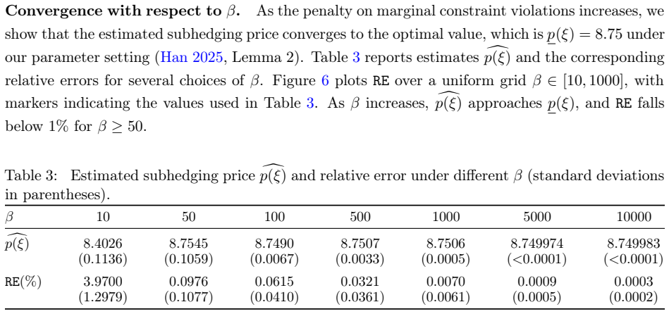
Scalable Bi-causal Optimal Transport via KL Relaxation and Policy Gradients
Pith reviewed 2026-05-19 23:06 UTC · model grok-4.3
pith:RPVPFU2J Add to your LaTeX paper
What is a Pith Number?\usepackage{pith}
\pithnumber{RPVPFU2J}
Prints a linked pith:RPVPFU2J badge after your title and writes the identifier into PDF metadata. Compiles on arXiv with no extra files. Learn more
The pith
KL relaxation turns bi-causal optimal transport into a policy-gradient problem
A machine-rendered reading of the paper's core claim, the machinery that carries it, and where it could break.
Core claim
We establish dynamic programming principles for both the original and relaxed formulations, prove that the relaxed problem converges to the original bi-causal OT problem as the penalty grows, and derive explicit policy-gradient representations for the relaxed objective. Building on these results, we propose a practical policy-gradient algorithm with unbiased mini-batch estimators, variance reduction, and nonasymptotic regret guarantees.
What carries the argument
The KL-penalized relaxation of the bi-causal optimal transport problem, which replaces hard marginal constraints with tractable divergence penalties while preserving recursive structure for dynamic programming and policy gradients.
If this is right
- Dynamic programming principles hold for the relaxed formulation.
- The relaxed problem converges to the original bi-causal OT as the penalty parameter grows.
- Explicit policy-gradient representations exist for the relaxed objective.
- The algorithm supplies unbiased mini-batch estimators, variance reduction, and nonasymptotic regret guarantees.
Where Pith is reading between the lines
- The framework could support generation of joint sample paths for simulation tasks that must respect both prescribed marginals and information flow over long horizons.
- Similar KL relaxations might extend to other sequential optimal transport problems that inherit a recursive structure.
- Integration with existing reinforcement learning optimizers could further reduce variance in high-dimensional path spaces.
Load-bearing premise
The KL relaxation preserves the recursive structure of the bi-causal problem sufficiently for dynamic programming and policy gradient methods to apply directly.
What would settle it
A calculation showing that the optimal value or couplings of the relaxed problem fail to approach those of the original bi-causal OT as the KL penalty tends to infinity would falsify the convergence claim.
Figures


read the original abstract
Bi-causal optimal transport (OT) is a natural framework for comparing and coupling stochastic processes under nonanticipative information constraints, with important applications in robust finance, sequential uncertainty quantification, and multistage stochastic optimization. In particular, a learned bi-causal coupling naturally serves as a simulator for generating joint sample paths that respect both prescribed marginal laws and the underlying information flow. Its practical use, however, is limited by the computational difficulty of enforcing bi-causal coupling constraints over path space, especially for continuous distributions and long horizons. We develop a scalable stochastic-optimization framework for computing bi-causal OT couplings under general marginals. Our approach introduces a Kullback--Leibler (KL)-penalized relaxation that replaces hard marginal constraints with tractable divergence penalties while preserving the recursive structure of the problem. We establish dynamic programming principles for both the original and relaxed formulations, prove that the relaxed problem converges to the original bi-causal OT problem as the penalty grows, and derive explicit policy-gradient representations for the relaxed objective. Building on these results, we propose a practical policy-gradient algorithm with unbiased mini-batch estimators, variance reduction, and nonasymptotic regret guarantees. Numerical experiments show that the method accurately captures marginal laws and temporal dependence, and performs well in applications including robust subhedging and time series statistical downscaling. These results provide a scalable computational approach to bi-causal OT and broaden its applicability in settings where nonanticipative information constraints are essential.
Editorial analysis
A structured set of objections, weighed in public.
Referee Report
Summary. The manuscript develops a scalable stochastic optimization framework for bi-causal optimal transport by replacing hard marginal constraints with a KL-penalized relaxation. It claims to establish dynamic programming principles for both the original and relaxed problems, prove convergence of the relaxed formulation to the original bi-causal OT as the penalty parameter tends to infinity, derive explicit policy-gradient representations for the relaxed objective, and introduce a practical algorithm using unbiased mini-batch estimators, variance reduction, and nonasymptotic regret guarantees. Numerical experiments illustrate accurate recovery of marginal laws and temporal dependence, with applications to robust subhedging and time-series downscaling.
Significance. If the central claims are rigorously established, the work offers a computationally tractable route to bi-causal couplings for continuous distributions and long horizons, which is valuable for robust finance, sequential uncertainty quantification, and multistage stochastic optimization. The combination of DP principles, convergence results, and regret bounds with a policy-gradient implementation would strengthen the practical utility of bi-causal OT beyond current limitations imposed by path-space constraints.
major comments (2)
- [Dynamic programming section for the relaxed formulation] The central derivation of dynamic programming for the relaxed problem (around the statement of the Bellman equation for the KL-penalized objective) assumes that the path-space KL divergence decomposes recursively with respect to the underlying filtration. A global KL term generally couples future and past information in a non-local manner; an explicit decomposition showing that the value function at each step depends only on the current state and conditional marginals is required to close the recursion and justify the subsequent policy-gradient and regret results.
- [Regret analysis and algorithm section] The nonasymptotic regret guarantees for the proposed policy-gradient algorithm (stated after the derivation of the gradient representations) depend on the unbiasedness of the mini-batch estimators and the variance reduction technique. The dependence of the regret bound on the time horizon T and the dimension of the state space should be made explicit, as this directly affects the claimed scalability for long-horizon problems.
minor comments (2)
- [Notation and preliminaries] Notation for the policy and the conditional marginals could be standardized between the original and relaxed formulations to improve readability.
- [Numerical experiments] The numerical experiments section would benefit from additional details on the choice of the KL penalty strength and its sensitivity in the reported results.
Simulated Author's Rebuttal
We sincerely thank the referee for the careful reading and constructive comments on our manuscript. We address each major comment point by point below and are prepared to revise the manuscript to incorporate the requested clarifications and strengthen the presentation.
read point-by-point responses
-
Referee: [Dynamic programming section for the relaxed formulation] The central derivation of dynamic programming for the relaxed problem (around the statement of the Bellman equation for the KL-penalized objective) assumes that the path-space KL divergence decomposes recursively with respect to the underlying filtration. A global KL term generally couples future and past information in a non-local manner; an explicit decomposition showing that the value function at each step depends only on the current state and conditional marginals is required to close the recursion and justify the subsequent policy-gradient and regret results.
Authors: We thank the referee for this observation. The KL relaxation in our formulation is constructed so that the divergence penalty is applied to the conditional distributions induced by the bi-causal policies with respect to the underlying filtration. This permits an exact recursive decomposition of the path-space KL term via the chain rule for relative entropy. Consequently, the value function at each time step depends only on the current state and the relevant conditional marginals, allowing the Bellman equation to close. We will add an explicit lemma (with full proof) detailing this decomposition immediately before the statement of the dynamic programming principle for the relaxed problem. revision: yes
-
Referee: [Regret analysis and algorithm section] The nonasymptotic regret guarantees for the proposed policy-gradient algorithm (stated after the derivation of the gradient representations) depend on the unbiasedness of the mini-batch estimators and the variance reduction technique. The dependence of the regret bound on the time horizon T and the dimension of the state space should be made explicit, as this directly affects the claimed scalability for long-horizon problems.
Authors: We agree that an explicit display of the dependence on the horizon T and state dimension is necessary for a transparent assessment of scalability. In the revised version we will restate the main regret theorem with all factors involving T and the dimension written out explicitly (the bound grows linearly in T and polynomially in dimension, modulated by the mini-batch size and variance-reduction parameters). We will also add a short remark discussing the implications for long-horizon regimes. revision: yes
Circularity Check
No significant circularity; derivations rest on standard DP and stochastic approximation
full rationale
The paper introduces a KL-penalized relaxation of bi-causal OT and claims to establish DP principles, convergence as penalty grows, and explicit policy-gradient representations. These steps are presented as following from the recursive structure preserved by the relaxation and from standard dynamic programming and policy gradient theory. No quoted equations reduce target quantities to fitted parameters defined within the paper, no load-bearing self-citations close the central claims, and no ansatz or uniqueness result is smuggled in via prior author work. The framework is therefore self-contained against external benchmarks for the purposes of this circularity check.
Axiom & Free-Parameter Ledger
free parameters (1)
- KL penalty strength
axioms (1)
- domain assumption Dynamic programming principle holds for both the original bi-causal OT and its KL relaxation
Lean theorems connected to this paper
-
IndisputableMonolith/Cost/FunctionalEquation.leanwashburn_uniqueness_aczel unclear?
unclearRelation between the paper passage and the cited Recognition theorem.
We establish dynamic programming principles for both the original and relaxed formulations... derive explicit policy-gradient representations for the relaxed objective.
-
IndisputableMonolith/Foundation/AlphaCoordinateFixation.leanJ_uniquely_calibrated_via_higher_derivative unclear?
unclearRelation between the paper passage and the cited Recognition theorem.
KL-penalized relaxation that replaces hard marginal constraints with tractable divergence penalties while preserving the recursive structure
What do these tags mean?
- matches
- The paper's claim is directly supported by a theorem in the formal canon.
- supports
- The theorem supports part of the paper's argument, but the paper may add assumptions or extra steps.
- extends
- The paper goes beyond the formal theorem; the theorem is a base layer rather than the whole result.
- uses
- The paper appears to rely on the theorem as machinery.
- contradicts
- The paper's claim conflicts with a theorem or certificate in the canon.
- unclear
- Pith found a possible connection, but the passage is too broad, indirect, or ambiguous to say the theorem truly supports the claim.
Reference graph
Works this paper leans on
-
[1]
For anyπ∈ΠΠΠbc, we haveQπ n+1 ∈Π n+1 for alln∈[N−1] 0, and J π n =c n +Q π n+1[J π n+1]≥c n +Q π n+1[Vn+1] = Γ Qπ n+1 n [Vn+1]≥Γ n[Vn+1]. Here, the first inequality follows fromJπ n+1 ≥V n+1 and the monotonicity of operatorQπ n+1, and the last inequality follows from (15). Then, by the definition ofVn in (13) as the infimum overπ∈ΠΠΠbc, we obtainVn ≥Γ n[Vn+1]
-
[2]
For anyϵ >0, there exist kernelsQ ϵ 1 ∈Π 1, . . . , Qϵ N ∈Π N such that for anyn∈[N−1] 0, Γn[Vn+1]≤c n +Q ϵ n+1[Vn+1]≤Γ n[Vn+1] +ϵ2 −(n+1) (A.1) Then, for anyπ0 ∈Π(µ 0, µ′ 0), we construct a Markov bi-causal coupling πϵ :=π π0,QQQϵ withQQQϵ = (Qϵ 1, . . . , Qϵ N).(A.2) 42 Next, we prove by backward induction that forn∈[N−1] 0, J πϵ n ≤Γ n[Vn+1] +ϵ N−1X k=...
-
[3]
For anyπ∈ΠΠΠbc withπ 0 ∈Π(µ 0, µ′ 0),J π 0 ≥V 0 and thus Eπ J π 0 (Y0, Y ′ 0) ≥E π V0(Y0, Y ′ 0) =E π0 V0(Y0, Y ′ 0) ≥inf π0∈Π(µ0,µ′ 0) Eπ0 V0(Y0, Y ′ 0) . 43 The definition ofWbc in (5) as the infimum overπ∈ΠΠΠbc yieldsW bc(µ, µ′)≥inf π0∈Π(µ0,µ′ 0) Eπ0[V0]
-
[4]
Notice that (A.3) holds for any initial coupling inΠ(µ0, µ′ 0)
For anyϵ >0, there existsγ ϵ 0 ∈Π(µ 0, µ′ 0)such that Eγϵ 0[V0]≤inf π0∈Π(µ0,µ′ 0) Eπ0[V0] +ϵ.(A.4) UsingQQQε defined in (A.2), we construct a Markov bi-causal couplingγϵ :=π γϵ 0,QQQε ∈ M bc. Notice that (A.3) holds for any initial coupling inΠ(µ0, µ′ 0). Therefore, Part I and (A.3) imply thatV 0 ≤J γϵ 0 < V0 +ϵ, and using (A.4), we have Eγϵ[J γϵ 0 ]≤E γϵ...
-
[5]
Eπ0[V0]. To establish the second equivalent representation, notice thatγ ϵ ∈ M bc(µ, µ′)⊂Π ΠΠbc and Wbc(µ, µ′) = inf π0∈Π(µ0,µ′
-
[6]
Eπ0[V0], we have Wbc(µ, µ′) = inf π∈ΠΠΠbc Eπ " NX n=0 cn(Yn, Y ′ n) # ≤inf π∈Mbc(µ,µ′) Eπ J π 0 (Y0, Y ′ 0) ≤E γϵ[J πϵ 0 (Y0, Y ′ 0)]≤W bc(µ, µ′) + 2ϵ.(A.5) Sinceϵ >0is arbitrary, all inequalities in (A.5) become equalities, and hence Wbc(µ, µ′) = inf π0∈Π(µ0,µ′ 0) Eπ0[V0(Y0, Y ′ 0)] = inf π∈Mbc(µ,µ′) Eπ " NX n=0 cn(Yn, Y ′ n) # .□ B Omitted proofs in Sec...
work page 2013
-
[7]
For anyπ∈Π rel, we considerQπ n+1 ∈ Urel for alln∈[N−1] 0, and eJ π n =c n +β h KL(1) n+1(µ, π) + KL(2) n+1(µ′, π) i +Q π n+1[eJ π n+1] ≥c n +β h KL(1) n+1(µ, π) + KL(2) n+1(µ′, π) i +Q π n+1[eVn+1] =eΓ Qπ n+1 n [eVn+1]≥ eΓn[eVn+1]. Here, the first inequality follows fromeJ π n+1 ≥ eVn+1 and the monotonicity of the operatorQπ n+1, and the last inequality ...
-
[8]
For anyϵ >0, there exist kernels eQϵ 1, . . . ,eQϵ N ∈ Urel such that for anyn∈[N−1] 0, eΓn[eVn+1]≤c n+β h KL(1) n+1(µ,eπϵ)+KL(2) n+1(µ′,eπϵ) i +eQϵ n+1[eVn+1]≤ eΓn[eVn+1]+ϵ2 −(n+1).(B.10) Then, for anyeπ0 ∈ P(S×S), we construct a relaxed Markov policy eπϵ :=π eπ0, eQeQeQϵ with eQeQeQϵ = (eQϵ 1, . . . ,eQϵ N).(B.11) 48 Next, we prove by backward induction...
-
[9]
Therefore, (17) is equivalent to Wrel(µ, µ′) = inf π∈Πrel Eπ0 h eJ π 0 (Y0, Y ′
+β KL(1) 0 (µ, π) + KL(2) 0 (µ′, π) i . Therefore, (17) is equivalent to Wrel(µ, µ′) = inf π∈Πrel Eπ0 h eJ π 0 (Y0, Y ′
-
[10]
To show the equivalent representation forWrel(µ, µ′), we combine the following two results
+β KL(1) 0 (µ, π) + KL(2) 0 (µ′, π) i . To show the equivalent representation forWrel(µ, µ′), we combine the following two results
-
[11]
For anyπ∈Π rel, we haveeJ π 0 ≥ eV0, and thus Eπ0 h eJ π 0 (Y0, Y ′
-
[12]
+β KL(1) 0 (µ, π) + KL(2) 0 (µ′, π) i ≥E π0 h eV0(Y0, Y ′
-
[13]
+β KL(1) 0 (µ, π) + KL(2) 0 (µ′, π) i ≥inf π0∈P(S×S) Eπ0 h eV0(Y0, Y ′
-
[14]
+β KL(1) 0 (µ, π) + KL(2) 0 (µ′, π) i . The definition ofWrel(µ, µ′)in (17) as the infimum overπ∈Π rel yields Wrel(µ, µ′)≥inf π0∈P(S×S) Eπ0 h eV0(Y0, Y ′
-
[15]
+β KL(1) 0 (µ, π) + KL(2) 0 (µ′, π) i
-
[16]
For anyϵ >0, there existseγϵ 0 ∈ P(S×S)such that Eeγϵ 0 h eV0(Y0, Y ′
-
[17]
+β KL(1) 0 (µ,eγϵ) + KL(2) 0 (µ′,eγϵ) i (B.14) ≤inf π0∈P(S×S) Eπ0 h eV0(Y0, Y ′
-
[18]
Using eQeQeQϵ defined in (B.11), we construct a relaxed Markov policy eγϵ :=π eγϵ 0, eQeQeQϵ ∈Π rel
+β KL(1) 0 (µ, π) + KL(2) 0 (µ′, π) i +ϵ. Using eQeQeQϵ defined in (B.11), we construct a relaxed Markov policy eγϵ :=π eγϵ 0, eQeQeQϵ ∈Π rel. Notice that (B.12) holds for any initial coupling inP(S×S). Therefore, Part I and (B.12) imply that eV0 ≤ eJ eγϵ 0 < eV0 +ϵ, which further gives that Eeγϵ 0 h eJ eγϵ 0 (Y0, Y ′
-
[19]
+β KL(1) 0 (µ,eγϵ) + KL(2) 0 (µ′,eγϵ) i ≤E eγϵ 0 h eV0(Y0, Y ′
-
[20]
+β KL(1) 0 (µ,eγϵ) + KL(2) 0 (µ′,eγϵ) i +ϵ 50 ≤inf π0∈P(S×S) Eπ0 h eV0(Y0, Y ′
-
[21]
+β KL(1) 0 (µ, π) + KL(2) 0 (µ′, π) i + 2ϵ, where the last inequality follows from (B.14). Therefore, by the definition ofWrel(µ, µ′)in (17) as the infimum overπ∈Π rel and the arbitrarily chosenϵ, we obtain Wrel(µ, µ′)≤inf π0∈P(S×S) Eπ0 h eV0(Y0, Y ′
-
[22]
+β KL(1) 0 (µ, π) + KL(2) 0 (µ′, π) i . Combining the two inequalities in both directions, we conclude that Wrel(µ, µ′) = inf π0∈P(S×S) Eπ0 h eV0(Y0, Y ′
-
[23]
NX k=0 ck( pYk, pY ′ k) ! ∇θn logq θn n ( pYn, pY ′ n | pYn−1, pY ′ n−1) # =E πθθθ
+β KL(1) 0 (µ, π) + KL(2) 0 (µ′, π) i .□ C Omitted proofs in Section 4 In this section, we provide the formal proofs of Theorems 2 and 3, Lemma 4, Corollary 1, and other supporting lemmas used in the proof. C.1 Proof of Theorem 2 Proof.In the following proof, we treatJval(θθθ)in (31) andJ KL(θθθ)in (32) separately. We consider the case with arbitraryn∈[N]...
work page 2021
discussion (0)
Sign in with ORCID, Apple, or X to comment. Anyone can read and Pith papers without signing in.