NPSolver: Neural Poisson Solver with Iterative Physics Supervision
Pith reviewed 2026-06-29 22:13 UTC · model grok-4.3
The pith
A neural network solves Poisson equations on irregular domains without labeled solutions by supervising itself with a few PCG iterations.
A machine-rendered reading of the paper's core claim, the machinery that carries it, and where it could break.
Core claim
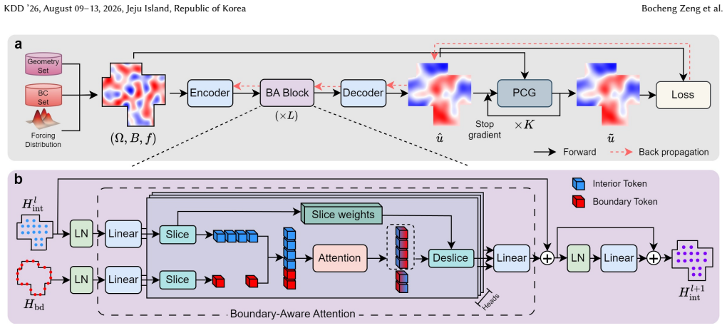
NPSolver is trained without solution labels via iterative physics supervision: a small number of preconditioned conjugate gradient steps refine the network's own predictions to produce a stable, well-scaled training signal. Theoretical analysis confirms that this supervision acts as a well-conditioned error proxy and that a stop-gradient design is essential for optimization stability. The Boundary-Aware Transolver architecture explicitly separates interior and boundary tokenization to capture boundary-driven features under mixed conditions.
What carries the argument
Iterative physics supervision that applies a small fixed number of preconditioned conjugate gradient steps to refine the model's predictions, together with the Boundary-Aware Transolver that tokenizes interior and boundary regions separately.
If this is right
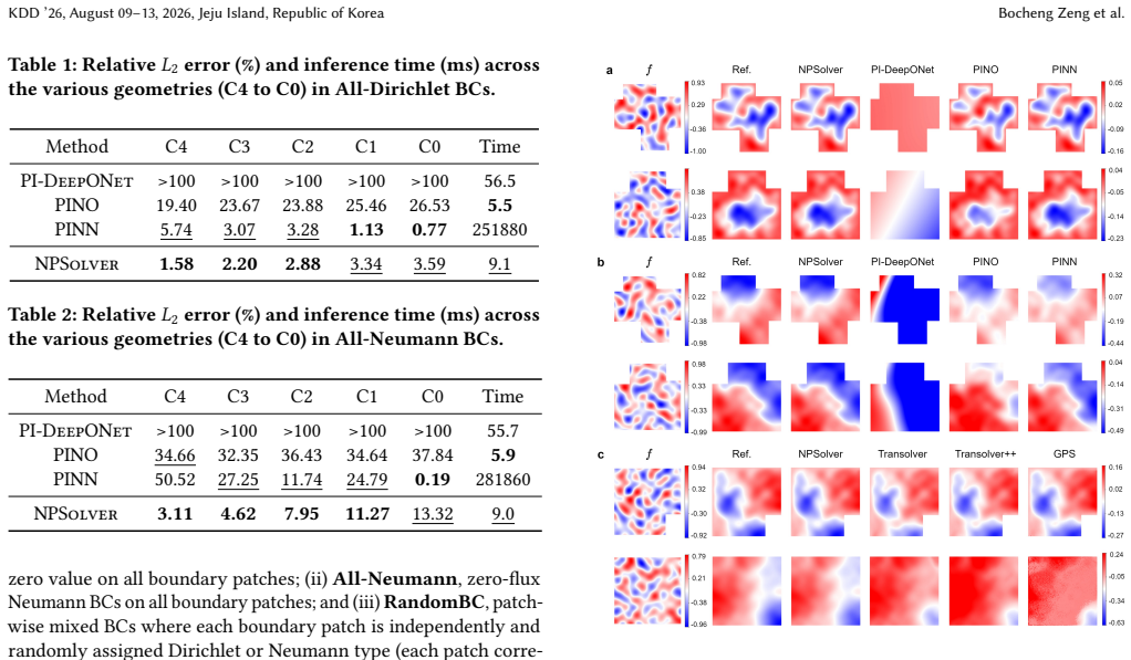
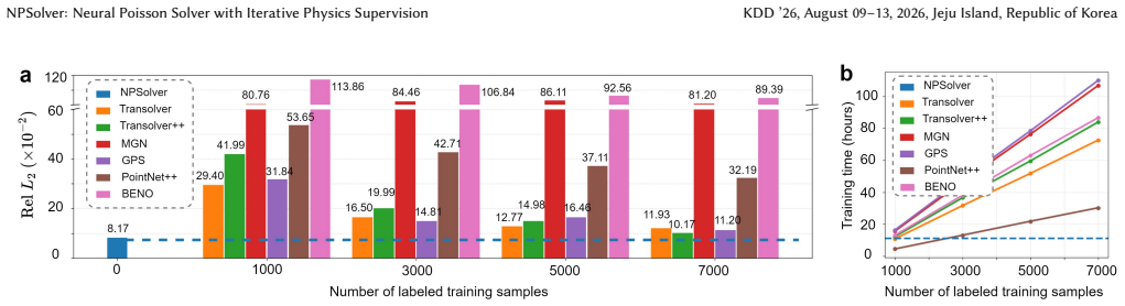
- The method outperforms both physics-informed and data-driven baselines on 2D and 3D irregular geometries.
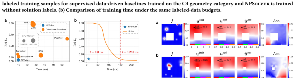
- A downstream thermal control task shows the model supports efficient gradient-based boundary control.
- The stop-gradient design prevents optimization instability during training.
- No labeled solution data or fully converged numerical solves are required at training time.
Where Pith is reading between the lines
- The same supervision pattern could be applied to other linear PDEs whose classical solvers are iterative but expensive to run to convergence.
- The interior-boundary token separation may improve accuracy for other boundary-value problems where boundaries dominate the solution.
- Hybrid use is possible in which the trained network supplies an initial guess that a classical solver then refines in very few steps.
Load-bearing premise
A small fixed number of PCG iterations supplies a sufficiently accurate and stable error proxy for training without ever needing fully converged numerical solutions or labeled data.
What would settle it
Training the network with the same small number of PCG steps yields predictions whose error does not decrease when the supervision is replaced by fully converged PCG solutions on the same geometries.
Figures

read the original abstract
Efficiently solving Poisson equations on complex, irregular domains remains a fundamental challenge in scientific computing, as classical iterative solvers often suffer from prohibitive runtime due to ill-conditioned systems. While neural operators offer a fast alternative, they typically rely on large-scale labeled datasets or struggle with unstable training dynamics when using physics-informed residual losses. We propose \textsc{NPSolver}, a neural Poisson solver trained without solution labels via iterative physics supervision. Instead of relying on fully converged numerical solutions or raw PDE residuals, \textsc{NPSolver} utilizes a small number of preconditioned conjugate gradient (PCG) steps to refine its own predictions, providing a more stable and well-scaled training signal. Theoretical analysis confirms that this iterative supervision serves as a well-conditioned error proxy and that a stop-gradient design is essential for optimization stability. To better capture boundary-driven features under mixed boundary conditions, we further introduce the Boundary-Aware Transolver (\textsc{BA-Transolver}) architecture that explicitly separates interior and boundary tokenization. Extensive evaluations on 2D and 3D irregular geometries demonstrate that \textsc{NPSolver} outperforms both physics-informed and data-driven baselines. Furthermore, a downstream thermal control task highlights the model's capability for conducting efficient and reliable gradient-based boundary control. We will release our codes and data at https://github.com/intell-sci-comput/NPSolver.
Editorial analysis
A structured set of objections, weighed in public.
Referee Report
Summary. The paper proposes NPSolver, a neural Poisson solver for 2D/3D irregular domains trained label-free via iterative physics supervision: a small fixed number of PCG steps refines the network's own predictions to yield a stable training signal, with stop-gradient required for optimization stability as confirmed by theoretical analysis. It introduces the Boundary-Aware Transolver (BA-Transolver) architecture that separates interior and boundary tokenization under mixed boundary conditions. Empirical evaluations on irregular geometries are claimed to outperform physics-informed and data-driven baselines, with an additional demonstration on a downstream thermal control task.
Significance. If the central claims hold, the work provides a concrete mechanism for stable, label-free training of neural PDE solvers that avoids both large labeled datasets and raw residual losses, while the boundary-aware architecture and downstream control example indicate applicability to practical scientific computing problems. The code release supports independent verification.
major comments (2)
- [Abstract, paragraph on iterative physics supervision] Abstract, paragraph on iterative physics supervision: the central assumption that a small fixed number of PCG iterations supplies a sufficiently accurate and stable error proxy without ever requiring fully converged numerical solutions is load-bearing for the label-free claim; the manuscript should report quantitative ablation on iteration count versus solution accuracy and training stability to substantiate that this proxy remains well-conditioned across the tested geometries.
- [Theoretical analysis] Theoretical analysis (referenced in abstract): while the stop-gradient design is stated to be essential for stability, the manuscript should explicitly connect the derived error-proxy conditioning bounds to the observed training dynamics (e.g., via a theorem or corollary that predicts the instability without stop-gradient) so that the necessity claim can be directly verified against the reported experiments.
minor comments (2)
- [Abstract] The abstract states that evaluations 'demonstrate that NPSolver outperforms both physics-informed and data-driven baselines' but does not preview the magnitude of improvement or the precise metrics; the results section should include a summary table with mean errors and standard deviations across all compared methods.
- Ensure that the released code repository contains the exact PCG preconditioner implementation, iteration counts, and random seeds used for the 2D/3D experiments so that the iterative supervision procedure can be reproduced exactly.
Simulated Author's Rebuttal
We thank the referee for the constructive feedback and the recommendation of minor revision. We address each major comment below and will update the manuscript accordingly.
read point-by-point responses
-
Referee: [Abstract, paragraph on iterative physics supervision] Abstract, paragraph on iterative physics supervision: the central assumption that a small fixed number of PCG iterations supplies a sufficiently accurate and stable error proxy without ever requiring fully converged numerical solutions is load-bearing for the label-free claim; the manuscript should report quantitative ablation on iteration count versus solution accuracy and training stability to substantiate that this proxy remains well-conditioned across the tested geometries.
Authors: We agree that a quantitative ablation on PCG iteration count would strengthen the central claim. In the revised manuscript we will add a new figure and table reporting solution accuracy (relative L2 error) and training stability (loss curves and final convergence) for iteration counts of 1, 5, 10 and 20 on both the 2D and 3D irregular-geometry benchmarks. These results will confirm that the small fixed count used in the main experiments remains well-conditioned. revision: yes
-
Referee: [Theoretical analysis] Theoretical analysis (referenced in abstract): while the stop-gradient design is stated to be essential for stability, the manuscript should explicitly connect the derived error-proxy conditioning bounds to the observed training dynamics (e.g., via a theorem or corollary that predicts the instability without stop-gradient) so that the necessity claim can be directly verified against the reported experiments.
Authors: We appreciate the suggestion to make the link between theory and experiment more explicit. We will add a short corollary in the theoretical analysis section that derives the divergence of the gradient signal in the absence of stop-gradient, directly referencing the conditioning bounds already obtained and showing consistency with the instability observed in our existing stop-gradient ablation experiments. revision: yes
Circularity Check
No significant circularity; derivation self-contained via external PCG
full rationale
The core training signal is generated by a fixed number of steps from the classical preconditioned conjugate gradient algorithm, an external numerical routine whose behavior is independent of the neural network parameters. The claimed theoretical analysis of the error proxy and stop-gradient necessity is presented as a separate derivation that does not reduce to a redefinition of the network output or to any fitted quantity internal to the model. No self-citation chain, ansatz smuggling, or renaming of known results is required for the central claim; the argument therefore remains non-circular and externally verifiable.
Axiom & Free-Parameter Ledger
Reference graph
Works this paper leans on
-
[1]
Zico Kolter, and Vladlen Koltun
Shaojie Bai, J. Zico Kolter, and Vladlen Koltun. 2019.Deep equilibrium models. Curran Associates Inc., Red Hook, NY, USA
2019
-
[2]
Briggs, Van Emden Henson, and Steve F
William L. Briggs, Van Emden Henson, and Steve F. McCormick. 2000.A Multi- grid Tutorial, Second Edition(second ed.). Society for Industrial and Applied Mathematics. doi:10.1137/1.9780898719505
-
[3]
Alexandre Joel Chorin. 1968. Numerical Solution of the Navier-Stokes Equations. Math. Comp.22, 104 (1968), 745–762
1968
-
[4]
Weinan E and Bing Yu. 2018. The Deep Ritz Method: A Deep Learning-Based Numerical Algorithm for Solving Variational Problems.Communications in Mathematics and Statistics6, 1 (01 Mar 2018), 1–12. https://doi.org/10.1007/ s40304-018-0127-z
2018
-
[5]
Karol Gregor and Yann LeCun. 2010. Learning fast approximations of sparse coding. InProceedings of the 27th International Conference on International Con- ference on Machine Learning(Haifa, Israel)(ICML’10). Omnipress, Madison, WI, USA, 399–406
2010
-
[6]
Tamara G Grossmann, Urszula Julia Komorowska, Jonas Latz, and Carola-Bibiane Schönlieb. 2024. Can physics-informed neural networks beat the finite element method?IMA Journal of Applied Mathematics89, 1 (2024), 143–174
2024
-
[7]
XU HAN, Han Gao, Tobias Pfaff, Jian-Xun Wang, and Liping Liu. 2022. Predict- ing Physics in Mesh-reduced Space with Temporal Attention. InInternational Conference on Learning Representations
2022
-
[8]
M. R. Hestenes and E. Stiefel. 1952. Methods of conjugate gradients for solving linear systems.Journal of research of the National Bureau of Standards49 (1952), 409–436
1952
-
[9]
Jun-Ting Hsieh, Shengjia Zhao, Stephan Eismann, Lucia Mirabella, and Stefano Ermon. 2019. Learning Neural PDE Solvers with Convergence Guarantees. In International Conference on Learning Representations
2019
-
[10]
J.D. Jackson. 1998.Classical Electrodynamics. Wiley
1998
-
[11]
Ameya D Jagtap and George Em Karniadakis. 2020. Extended physics-informed neural networks (xpinns): A generalized space-time domain decomposition based deep learning framework for nonlinear partial differential equations.Communi- cations in Computational Physics28, 5 (2020), 2002–2041
2020
-
[12]
E. Kharazmi, Z. Zhang, and G. E. Karniadakis. 2019. Variational Physics- Informed Neural Networks For Solving Partial Differential Equations. arXiv:1912.00873 [cs.NE]
-
[13]
Ehsan Kharazmi, Zhongqiang Zhang, and George E.M. Karniadakis. 2021. hp- VPINNs: Variational physics-informed neural networks with domain decomposi- tion.Computer Methods in Applied Mechanics and Engineering374 (2021), 113547. doi:10.1016/j.cma.2020.113547
-
[14]
Aditi Krishnapriyan, Amir Gholami, Shandian Zhe, Robert Kirby, and Michael W Mahoney. 2021. Characterizing possible failure modes in physics-informed neural networks.Advances in neural information processing systems34 (2021), 26548– 26560
2021
-
[15]
Randall J. LeVeque. 2007.Finite Difference Methods for Ordinary and Partial Differential Equations. Society for Industrial and Applied Mathematics. doi:10. 1137/1.9780898717839
2007
-
[16]
Tianyu Li, Yiye Zou, Shufan Zou, Xinghua Chang, Laiping Zhang, and Xiaogang Deng. 2024. A fully differentiable GNN-based PDE Solver: With Applications to Poisson and Navier-Stokes Equations. (2024). KDD ’26, August 09–13, 2026, Jeju Island, Republic of Korea Bocheng Zeng et al
2024
-
[17]
Zongyi Li, Daniel Zhengyu Huang, Burigede Liu, and Anima Anandkumar. 2023. Fourier Neural Operator with Learned Deformations for PDEs on General Ge- ometries.Journal of Machine Learning Research24, 388 (2023), 1–26
2023
-
[18]
Zongyi Li, Nikola Borislavov Kovachki, Kamyar Azizzadenesheli, Burigede liu, Kaushik Bhattacharya, Andrew Stuart, and Anima Anandkumar. 2021. Fourier Neural Operator for Parametric Partial Differential Equations. InInternational Conference on Learning Representations
2021
-
[19]
Zongyi Li, Nikola Borislavov Kovachki, Chris Choy, Boyi Li, Jean Kossaifi, Shourya Prakash Otta, Mohammad Amin Nabian, Maximilian Stadler, Christian Hundt, Kamyar Azizzadenesheli, and Anima Anandkumar. 2023. Geometry- Informed Neural Operator for Large-Scale 3D PDEs. InThirty-seventh Conference on Neural Information Processing Systems
2023
-
[20]
Zijie Li, Kazem Meidani, and Amir Barati Farimani. 2023. Transformer for Partial Differential Equations’ Operator Learning.Transactions on Machine Learning Research(2023)
2023
-
[21]
Zhihao Li, Haoze Song, Di Xiao, Zhilu Lai, and Wei Wang. 2025. Harnessing Scale and Physics: A Multi-Graph Neural Operator Framework for PDEs on Arbitrary Geometries. InProceedings of the 31st ACM SIGKDD Conference on Knowledge Discovery and Data Mining V.1(Toronto ON, Canada)(KDD ’25). Association for Computing Machinery, New York, NY, USA, 729–740. doi:...
-
[22]
Zongyi Li, Hongkai Zheng, Nikola Kovachki, David Jin, Haoxuan Chen, Burigede Liu, Kamyar Azizzadenesheli, and Anima Anandkumar. 2024. Physics-Informed Neural Operator for Learning Partial Differential Equations.ACM / IMS J. Data Sci.1, 3, Article 9 (May 2024), 27 pages. doi:10.1145/3648506
-
[23]
Lu Lu, Pengzhan Jin, Guofei Pang, Zhongqiang Zhang, and George Em Karni- adakis. 2021. Learning nonlinear operators via DeepONet based on the universal approximation theorem of operators.Nature Machine Intelligence3, 3 (2021), 218–229
2021
-
[24]
Lu Lu, Xuhui Meng, Shengze Cai, Zhiping Mao, Somdatta Goswami, Zhongqiang Zhang, and George Em Karniadakis. 2022. A comprehensive and fair comparison of two neural operators (with practical extensions) based on FAIR data.Computer Methods in Applied Mechanics and Engineering393 (2022), 114778. doi:10.1016/j. cma.2022.114778
work page doi:10.1016/j 2022
-
[25]
Huakun Luo, Haixu Wu, Hang Zhou, Lanxiang Xing, Yichen Di, Jianmin Wang, and Mingsheng Long. 2025. Transolver++: An Accurate Neural Solver for PDEs on Million-Scale Geometries. InInternational Conference on Machine Learning
2025
-
[26]
F. Moukalled, L. Mangani, and M. Darwish. 2016.The Finite Volume Method in Computational Fluid Dynamics : An Advanced Introduction with OpenFOAM® and Matlab. Fluid Mechanics and its Applications, Vol. 113. Springer, Cham. doi:10.1007/978-3-319-16874-6
-
[27]
Ruben Ohana, Michael McCabe, Lucas Meyer, Rudy Morel, Fruzsina Agocs, Miguel Beneitez, Marsha Berger, Blakesly Burkhart, Stuart Dalziel, Drummond Fielding, et al. 2024. The well: a large-scale collection of diverse physics simula- tions for machine learning.Advances in Neural Information Processing Systems 37 (2024), 44989–45037
2024
-
[28]
1980.Numerical heat transfer and fluid flow
Suhas V Patankar. 1980.Numerical heat transfer and fluid flow. Hemisphere Publishing Corporation (CRC Press, Taylor & Francis Group)
1980
-
[29]
Tobias Pfaff, Meire Fortunato, Alvaro Sanchez-Gonzalez, and Peter Battaglia
-
[30]
InInternational Conference on Learning Representations
Learning Mesh-Based Simulation with Graph Networks. InInternational Conference on Learning Representations
-
[31]
Qi, Li Yi, Hao Su, and Leonidas J
Charles R. Qi, Li Yi, Hao Su, and Leonidas J. Guibas. 2017. PointNet++: deep hierarchical feature learning on point sets in a metric space. InProceedings of the 31st International Conference on Neural Information Processing Systems(Long Beach, California, USA)(NIPS’17). Curran Associates Inc., Red Hook, NY, USA, 5105–5114
2017
-
[32]
Md Ashiqur Rahman, Zachary E Ross, and Kamyar Azizzadenesheli. 2023. U-NO: U-shaped Neural Operators.Transactions on Machine Learning Research(2023)
2023
-
[33]
Maziar Raissi. 2018. Deep hidden physics models: deep learning of nonlinear partial differential equations.J. Mach. Learn. Res.19, 1 (jan 2018), 932–955
2018
-
[34]
M. Raissi, P. Perdikaris, and G.E. Karniadakis. 2019. Physics-informed neural networks: A deep learning framework for solving forward and inverse problems involving nonlinear partial differential equations.J. Comput. Phys.378 (2019), 686–707. doi:10.1016/j.jcp.2018.10.045
-
[35]
Ladislav Rampášek, Mikhail Galkin, Vijay Prakash Dwivedi, Anh Tuan Luu, Guy Wolf, and Dominique Beaini. 2022. Recipe for a General, Powerful, Scalable Graph Transformer.Advances in Neural Information Processing Systems35 (2022)
2022
-
[36]
2003.Iterative Methods for Sparse Linear Systems(second ed.)
Yousef Saad. 2003.Iterative Methods for Sparse Linear Systems(second ed.). Society for Industrial and Applied Mathematics. doi:10.1137/1.9780898718003
-
[37]
Justin Sirignano and Konstantinos Spiliopoulos. 2018. DGM: A deep learning algorithm for solving partial differential equations.J. Comput. Phys.375 (2018), 1339–1364. doi:10.1016/j.jcp.2018.08.029
-
[38]
Alasdair Tran, Alexander Mathews, Lexing Xie, and Cheng Soon Ong. 2023. Factorized Fourier Neural Operators. InThe Eleventh International Conference on Learning Representations
2023
-
[39]
Oosterlee, and Anton Schüller
Ulrich Trottenberg, Cornelis W. Oosterlee, and Anton Schüller. 2001.Multigrid. Texts in Applied Mathematics. Bd., Vol. 33. Academic Press, San Diego [u.a.]. With contributions by A. Brandt, P. Oswald and K. Stüben
2001
-
[40]
Han Wan, Qi Wang, Yuan Mi, Rui Zhang, and Hao Sun. 2026. PIMRL: Physics- Informed Multi-Scale Recurrent Learning for Burst-Sampled Spatiotemporal Dynamics.Proceedings of the AAAI Conference on Artificial Intelligence40 (Mar. 2026), 1096–1104. doi:10.1609/aaai.v40i2.37080
-
[41]
Haixin Wang, Jiaxin LI, Anubhav Dwivedi, Kentaro Hara, and Tailin Wu. 2024. BENO: Boundary-embedded Neural Operators for Elliptic PDEs. InThe Twelfth International Conference on Learning Representations
2024
-
[42]
Sifan Wang, Hanwen Wang, and Paris Perdikaris. 2021. Learning the solution operator of parametric partial differential equations with physics-informed Deep- ONets.Science Advances7, 40 (2021), eabi8605. doi:10.1126/sciadv.abi8605
-
[43]
Sifan Wang, Xinling Yu, and Paris Perdikaris. 2022. When and why PINNs fail to train: A neural tangent kernel perspective.J. Comput. Phys.449 (2022), 110768
2022
-
[44]
Haixu Wu, Huakun Luo, Haowen Wang, Jianmin Wang, and Mingsheng Long
-
[45]
In International Conference on Machine Learning
Transolver: A Fast Transformer Solver for PDEs on General Geometries. In International Conference on Machine Learning
-
[46]
Jeremy Yu, Lu Lu, Xuhui Meng, and George Em Karniadakis. 2022. Gradient- enhanced physics-informed neural networks for forward and inverse PDE prob- lems.Computer Methods in Applied Mechanics and Engineering393 (2022), 114823. doi:10.1016/j.cma.2022.114823
-
[47]
Bocheng Zeng, Qi Wang, Mengtao Yan, Yang Liu, Ruizhi Chengze, Yi Zhang, Hongsheng Liu, Zidong Wang, and Hao Sun. 2025. PhyMPGN: Physics-encoded Message Passing Graph Network for spatiotemporal PDE systems. InThe Thir- teenth International Conference on Learning Representations
2025
-
[48]
Enrui Zhang, Adar Kahana, Alena Kopaničáková, Eli Turkel, Rishikesh Ranade, Jay Pathak, and George Em Karniadakis. 2024. Blending neural operators and relaxation methods in PDE numerical solvers.Nature Machine Intelligence6, 11 (01 Nov 2024), 1303–1313. doi:10.1038/s42256-024-00910-x
-
[49]
Rui Zhang, Qi Meng, Han Wan, Yang Liu, Zhi-Ming Ma, and Hao Sun
-
[50]
arXiv:2506.10862 [physics.flu-dyn]
OmniFluids: Physics Pre-trained Modeling of Fluid Dynamics. arXiv:2506.10862 [physics.flu-dyn]
-
[51]
Rui Zhang, Qi Meng, Rongchan Zhu, Yue Wang, Wenlei Shi, Shihua Zhang, Zhi- Ming Ma, and Tie-Yan Liu. 2025. Monte carlo neural pde solver for learning pdes via probabilistic representation.IEEE Transactions on Pattern Analysis and Machine Intelligence(2025)
2025
-
[52]
Zienkiewicz and R.L
O.C. Zienkiewicz and R.L. Taylor. 2013.The Finite Element Method: Its Basis and Fundamentals. Butterworth-Heinemann. Appendix A FVM Discretization We adopt a cell-centered finite-volume method (FVM) to discretize the Poisson equation on an irregular domain. As illustrated in Fig. A.1, the computational domain is partitioned into a set of non- overlapping ...
2013
-
[53]
hot spots
∈ [0,1). Lemma C.1 (Norm eqivalence under symmetric precon- ditioning).Let 𝒚=𝑴 1/2𝒖 and 𝒚★ =𝑴 1/2𝒖★. Then 𝒚★ solves 𝑪𝒚=𝑴 −1/2𝒃, and for any𝒖, ∥𝒖−𝒖 ★∥𝑨 =∥𝒚−𝒚 ★∥𝑪 . Proof. We have 𝑨𝒖=𝒃⇐ ⇒𝑴 −1/2𝑨𝑴 −1/2𝒚=𝑴 −1/2𝒃, i.e., 𝑪𝒚=𝑴 −1/2𝒃. Moreover, ∥𝒖−𝒖 ★∥2 𝑨 =(𝒖−𝒖 ★)⊤𝑨(𝒖−𝒖 ★) =(𝒚−𝒚 ★)⊤𝑴 −1/2𝑨𝑴 −1/2 (𝒚−𝒚 ★) =∥𝒚−𝒚 ★∥2 𝑪 . □ Lemma C.2 (Kantorovich ineqality).Let 𝑪 be S...
2026
-
[54]
Number of hot spots: 𝐾∼Unif{𝐾 min, 𝐾max}
-
[55]
from {1,
Hot-spot centers: we sample 𝐾 indices {𝑐𝑘 }𝐾 𝑘=1 i.i.d. from {1, . . . , 𝑛}, and set 𝝁𝑘 =𝒙 𝑐𝑘 =(𝜇 𝑘,𝑥 , 𝜇𝑘,𝑦 )
-
[56]
and we use isotropic widths 𝜎𝑘,𝑥 =𝜎 𝑘,𝑦 =𝑠 𝑘
Amplitudes and widths: 𝐴𝑘 ∼Unif(𝑎 min, 𝑎max), 𝑠 𝑘 ∼Unif(𝑠 min, 𝑠max), Figure A.4: Relationship between the estimated condition number and the relative 𝐿2 error gap between residual super- vision and iterative supervision on C4. and we use isotropic widths 𝜎𝑘,𝑥 =𝜎 𝑘,𝑦 =𝑠 𝑘
-
[57]
Unnormalized field: for each point𝒙 𝑖 =(𝑥 𝑖, 𝑦𝑖 ), 𝑓0 (𝒙𝑖 )= 𝐾∑︁ 𝑘=1 𝐴𝑘 exp − 1 2 𝑥𝑖 −𝜇 𝑘,𝑥 𝜎𝑘,𝑥 +𝜀 2 − 1 2 𝑦𝑖 −𝜇 𝑘,𝑦 𝜎𝑘,𝑦 +𝜀 2! , 𝜀=10 −8
-
[58]
Then the returned heat-source field is scaled: 𝑓(𝒙 𝑖 )=𝑓 0 (𝒙𝑖 ) · 1 ¯𝑓0 +𝜀
Mean-power scaling: define the sample mean ¯𝑓0 = 1 𝑛 𝑛∑︁ 𝑖=1 𝑓0 (𝒙𝑖 ). Then the returned heat-source field is scaled: 𝑓(𝒙 𝑖 )=𝑓 0 (𝒙𝑖 ) · 1 ¯𝑓0 +𝜀 . In practice, we choose 𝐾min = 2, 𝐾max = 6, 𝑎min = 0.5, 𝑎max = 2.0, 𝑠min = 0.02𝐿, 𝑠max = 0.08𝐿, 𝐿= 2𝜋 to produce spatially sparse, inhomogeneous sources that resemble heat injection from discrete components. F...
2026
discussion (0)
Sign in with ORCID, Apple, or X to comment. Anyone can read and Pith papers without signing in.