pith. sign in

arxiv: 2605.29283 · v2 · pith:SS4EM4JNnew · submitted 2026-05-28 · 💻 cs.LG · cs.AI

Do Physics Foundation Models Learn Generalizable Physics? A Bias-Aware Benchmark Across Physical Regimes and Distribution Shifts

Pith reviewed 2026-07-04 00:37 UTC · model grok-4.3

classification 💻 cs.LG cs.AI
keywords physics foundation modelsspatiotemporal forecastingdistribution shiftsbenchmark evaluationmodel generalityconditional performancepretraining effects
0
0 comments X

The pith

Physics foundation models perform as conditional generalists whose success depends on regime, temporal scale, and initial conditions rather than as universal predictors.

A machine-rendered reading of the paper's core claim, the machinery that carries it, and where it could break.

The paper builds a benchmark spanning eight physical dynamics, three training-data mixtures, and twenty-five test regimes created by dynamic-scale and initial-condition complexity shifts. These regimes cover in-distribution, distribution-shift, and out-of-distribution cases and are used to run sixty thousand measurements on five architectures each with four variants. The measurements show that model performance varies systematically with physical regime, temporal scale, initial-condition setting, pretraining status, model size, and architecture. Expanding the training distribution yields only partial relief, and neither pretraining nor scaling removes the observed ability biases. The authors conclude that future progress requires learning mechanisms that capture transferable physical knowledge across regimes and shifts rather than relying on scale alone.

Core claim

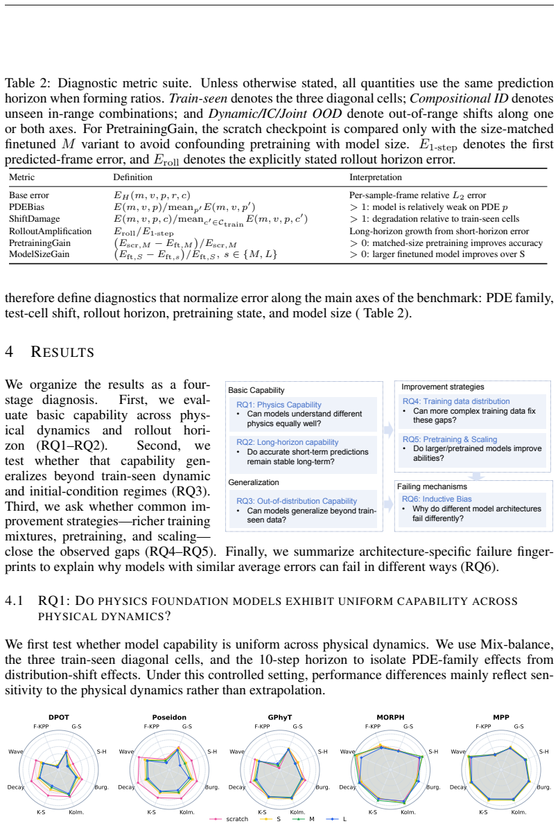
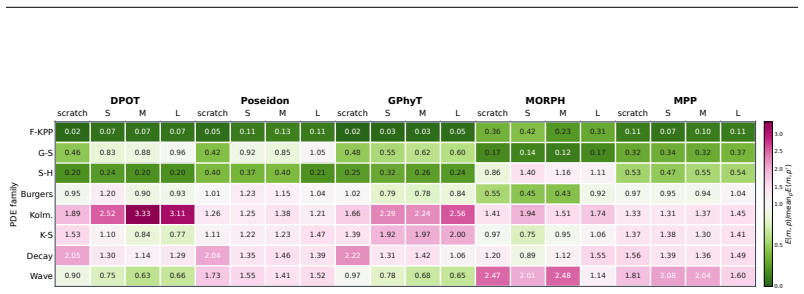
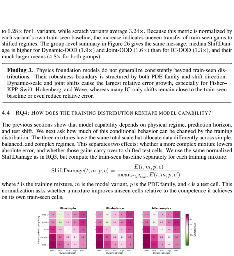
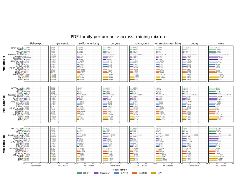
Current physics foundation models behave as conditional rather than universal generalists: their generality depends on the physical regime, temporal scale, initial-condition setting, pretraining, model size, and architecture. Improving the training data distribution only partially mitigates this limitation. Pretraining and scaling are also unable to reliably remove their ability biases.

What carries the argument

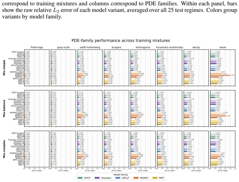
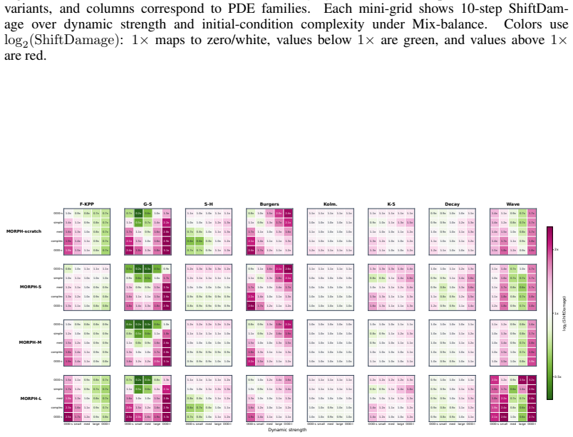
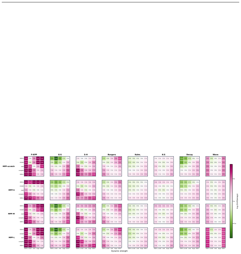
The benchmark of eight physical dynamics, three training-data mixtures, and twenty-five test regimes induced by dynamic-scale and initial-condition complexity shifts that produces sixty thousand measurements across model variants.

Load-bearing premise

The twenty-five test regimes induced by dynamic-scale and initial-condition complexity shifts sufficiently represent the distribution shifts that matter for real-world use.

What would settle it

A single physics foundation model that maintains high accuracy across all twenty-five regimes irrespective of pretraining, size, or architecture would falsify the conditional-generality claim.

Figures

Figures reproduced from arXiv: 2605.29283 by Ayan Biswas, Han-Wei Shen, Mengdi Chu, Yang Liu.

Figure 1
Figure 1. Figure 1: Overview of the benchmark protocol. The evaluation space is organized as a [PITH_FULL_IMAGE:figures/full_fig_p003_1.png] view at source ↗
Figure 2
Figure 2. Figure 2: Raw PDE performance. Each plot corresponds to one model family, and each curve shows one model variant: scratch, S, M, and L. The eight axes denote PDE families, and the plotted value is the raw relative L2 error averaged over the three train-seen cells and the 10 in-horizon predicted frames. Lower values indicate better absolute accuracy. The radial axis is shown on a log scale to make both low-error and … view at source ↗
Figure 3
Figure 3. Figure 3: PDEBias. Rows correspond to PDE families and columns correspond to model vari￾ants, grouped by architecture and variant type. Each cell reports the within-model normalized error E(m, p)/meanp′E(m, p′ ), computed using relative L2 error averaged over the three train-seen cells and the 10 in-horizon predicted frames. Values below 1 indicate PDE families on which a model is relatively stronger than its own av… view at source ↗
Figure 4
Figure 4. Figure 4: PDE-wise rollout error growth. Each subplot is one PDE family. Curves show the frame￾wise relative L2 error of all model variants, with colors grouped by architecture and shade indicating scratch/S/M/L variants. The gray region marks frames beyond the 10-step training horizon. Errors generally grow with prediction time, but the growth pattern depends strongly on both PDE family and model variant. scratch S… view at source ↗
Figure 5
Figure 5. Figure 5: 10-step in-horizon error amplification by model variant and PDE family. Rows cor￾respond to PDE families and columns correspond to model variants, grouped by architecture and variant type. Each cell reports E10-step/E1-step, where E1-step is the first predicted-frame error and E10-step is the average error over the 10 in-horizon predicted frames. Larger values indicate stronger error accumulation within th… view at source ↗
Figure 6
Figure 6. Figure 6: PDE-wise 5×5 ShiftDamage grids under Mix-balance. Each panel corresponds to one PDE family, computed at the 10-step horizon. Columns increase dynamic strength from OOD￾small to OOD-large, and rows increase initial-condition complexity from OOD-simple to OOD￾complex. Each cell reports ShiftDamage averaged over all evaluated model variants, with each variant normalized by its own train-seen diagonal baseline… view at source ↗
Figure 7
Figure 7. Figure 7: Training-mixture effect on the 5 × 5 ShiftDamage grid. Each panel corresponds to one training mixture. Rows vary initial-condition complexity and columns vary dynamic scale. Each cell reports mean normalized ShiftDamage averaged over model variants and PDE families, using the 10-step relative L2 error. Colors use log2 (ShiftDamage): 1× maps to white, values below 1× are green, and values above 1× are red … view at source ↗
Figure 8
Figure 8. Figure 8: Matched-size PretrainingGain under Mix-balance. Rows correspond to PDE fami￾lies and columns correspond to architectures. Each cell reports the percentage error reduction of pretrained-M relative to scratch-M for the same architecture, averaged over the full 25-cell grid at the 10-step horizon. Green indicates beneficial transfer and pink indicates negative transfer. S M L S M L S M L S M L S M L F-KPP G-S… view at source ↗
Figure 9
Figure 9. Figure 9: ModelSizeGain under Mix-balance. Rows correspond to PDE families and columns correspond to model variants, grouped by architecture and finetuned size. Each cell reports the percentage error reduction relative to the S finetuned model of the same architecture and PDE. The S column is therefore zero. Green indicates that the larger model improves over S; pink indicates inverse scaling. Finding 5. Pretraining… view at source ↗
Figure 10
Figure 10. Figure 10: Architecture-level failure-mechanism fingerprint. Rows correspond to architectures and columns correspond to failure dimensions derived from the diagnostics above. Values are min– max normalized within each column, so darker cells indicate that an architecture is relatively more affected by that failure mode. remains affected by PDE and rollout variation. These differences indicate that architecture matte… view at source ↗
Figure 11
Figure 11. Figure 11: Gray–Scott examples. Rows are IC families ordered from OOD-simple to OOD [PITH_FULL_IMAGE:figures/full_fig_p016_11.png] view at source ↗
Figure 12
Figure 12. Figure 12: Wave-equation examples. Rows are IC families ordered from OOD-simple to OOD [PITH_FULL_IMAGE:figures/full_fig_p016_12.png] view at source ↗
Figure 13
Figure 13. Figure 13: Fisher–KPP examples. Rows are IC families ordered from OOD-simple to OOD [PITH_FULL_IMAGE:figures/full_fig_p017_13.png] view at source ↗
Figure 14
Figure 14. Figure 14: Burgers examples. Rows are IC families ordered from OOD-simple to OOD-complex; [PITH_FULL_IMAGE:figures/full_fig_p018_14.png] view at source ↗
Figure 15
Figure 15. Figure 15: Swift–Hohenberg examples. Rows are IC families ordered from OOD-simple to OOD [PITH_FULL_IMAGE:figures/full_fig_p018_15.png] view at source ↗
Figure 16
Figure 16. Figure 16: Navier–Stokes decay examples. Rows are IC families ordered from OOD-simple to [PITH_FULL_IMAGE:figures/full_fig_p019_16.png] view at source ↗
Figure 17
Figure 17. Figure 17: Kolmogorov-flow examples. Rows are IC families ordered from OOD-simple to OOD [PITH_FULL_IMAGE:figures/full_fig_p019_17.png] view at source ↗
Figure 18
Figure 18. Figure 18: Kuramoto–Sivashinsky examples. Rows are IC families ordered from OOD-simple to [PITH_FULL_IMAGE:figures/full_fig_p020_18.png] view at source ↗
Figure 19
Figure 19. Figure 19: PDE-family raw error across training mixtures at the first predicted frame. Rows correspond to training mixtures and columns correspond to PDE families. Within each panel, bars show the raw relative L2 error of each model variant, averaged over all 25 test regimes. Colors group variants by model family. MPP-L MPP-M MPP-S MPP-scratch MORPH-L MORPH-M MORPH-S MORPH-scratch GPhyT-L GPhyT-M GPhyT-S GPhyT-scrat… view at source ↗
Figure 20
Figure 20. Figure 20: PDE-family raw error across training mixtures at the 10-step horizon. Rows corre￾spond to training mixtures and columns correspond to PDE families. Within each panel, bars show the raw relative L2 error of each model variant, averaged over all 25 test regimes and the 10 in￾horizon predicted frames. Colors group variants by model family. 21 [PITH_FULL_IMAGE:figures/full_fig_p021_20.png] view at source ↗
Figure 21
Figure 21. Figure 21: PDE-family raw error across training mixtures over the full 15-frame rollout. Rows correspond to training mixtures and columns correspond to PDE families. Within each panel, bars show the raw relative L2 error of each model variant, averaged over all 25 test regimes and all 15 predicted frames. Colors group variants by model family. scratch S M L scratch S M L scratch S M L scratch S M L scratch S M L F-K… view at source ↗
Figure 22
Figure 22. Figure 22: 15th-frame rollout amplification by model variant and PDE family. Each cell reports E15th-frame/E1st-frame, where E15th-frame is the error at prediction frame 15 and E1st-frame is the first predicted-frame error. This figure is the rollout-horizon counterpart of [PITH_FULL_IMAGE:figures/full_fig_p022_22.png] view at source ↗
Figure 23
Figure 23. Figure 23: Raw first-frame error by model variant and PDE family. Each cell reports the raw relative L2 error at prediction frame 1, averaged over the three train-seen cells under Mix-balance. Rows correspond to PDE families and columns correspond to model variants. The OrRd color range is normalized using the minimum and maximum values within this figure. 22 [PITH_FULL_IMAGE:figures/full_fig_p022_23.png] view at source ↗
Figure 24
Figure 24. Figure 24: Raw 10th-frame error by model variant and PDE family. Each cell reports the raw relative L2 error at prediction frame 10, averaged over the three train-seen cells under Mix-balance. Rows correspond to PDE families and columns correspond to model variants. The OrRd color range is normalized using the minimum and maximum values within this figure. scratch S M L scratch S M L scratch S M L scratch S M L scra… view at source ↗
Figure 25
Figure 25. Figure 25: Raw 15th-frame error by model variant and PDE family. Each cell reports the raw relative L2 error at prediction frame 15, averaged over the three train-seen cells under Mix-balance. Rows correspond to PDE families and columns correspond to model variants. The OrRd color range is normalized using the minimum and maximum values within this figure. Train Comp. Dyn-OOD IC-OOD Joint 10 0 10 1 ShiftDamage F-KPP… view at source ↗
Figure 26
Figure 26. Figure 26: ShiftDamage by shift group. The same 10-step grouping shown separately for each PDE family. The dashed line marks no degradation relative to the train-seen baseline. Dynamic-OOD and Joint-OOD have the heaviest tails, indicating that dynamic-scale extrapolation produces larger relative robustness gaps than IC-only shifts on average, although the severity is PDE-dependent. 23 [PITH_FULL_IMAGE:figures/full_… view at source ↗
Figure 27
Figure 27. Figure 27: DPOT variant-level 5 × 5 ShiftDamage grids. Rows correspond to scratch/S/M/L variants, and columns correspond to PDE families. Each mini-grid shows 10-step ShiftDam￾age over dynamic strength and initial-condition complexity under Mix-balance. Colors use log2 (ShiftDamage): 1× maps to zero/white, values below 1× are green, and values above 1× are red. OOD-s simple med complex OOD-c Poseidon-scratch 2.1x 1.… view at source ↗
Figure 28
Figure 28. Figure 28: Poseidon variant-level 5 × 5 ShiftDamage grids. Rows correspond to scratch/S/M/L variants, and columns correspond to PDE families. Each mini-grid shows 10-step ShiftDam￾age over dynamic strength and initial-condition complexity under Mix-balance. Colors use log2 (ShiftDamage): 1× maps to zero/white, values below 1× are green, and values above 1× are red. 24 [PITH_FULL_IMAGE:figures/full_fig_p024_28.png] view at source ↗
Figure 29
Figure 29. Figure 29: GPhyT variant-level 5 × 5 ShiftDamage grids. Rows correspond to scratch/S/M/L variants, and columns correspond to PDE families. Each mini-grid shows 10-step ShiftDam￾age over dynamic strength and initial-condition complexity under Mix-balance. Colors use log2 (ShiftDamage): 1× maps to zero/white, values below 1× are green, and values above 1× are red. OOD-s simple med complex OOD-c MORPH-scratch 1.0x 0.9x… view at source ↗
Figure 30
Figure 30. Figure 30: MORPH variant-level 5 × 5 ShiftDamage grids. Rows correspond to scratch/S/M/L variants, and columns correspond to PDE families. Each mini-grid shows 10-step ShiftDam￾age over dynamic strength and initial-condition complexity under Mix-balance. Colors use log2 (ShiftDamage): 1× maps to zero/white, values below 1× are green, and values above 1× are red. 25 [PITH_FULL_IMAGE:figures/full_fig_p025_30.png] view at source ↗
Figure 31
Figure 31. Figure 31: MPP variant-level 5 × 5 ShiftDamage grids. Rows correspond to scratch/S/M/L variants, and columns correspond to PDE families. Each mini-grid shows 10-step ShiftDam￾age over dynamic strength and initial-condition complexity under Mix-balance. Colors use log2 (ShiftDamage): 1× maps to zero/white, values below 1× are green, and values above 1× are red. 26 [PITH_FULL_IMAGE:figures/full_fig_p026_31.png] view at source ↗
read the original abstract

Recent physics foundation models claim general spatiotemporal forecasting ability, yet their evaluations often collapse performance into a single average score under a fixed training distribution. This makes it difficult to determine whether a model has learned generalizable physical dynamics or only performs well under particular settings. We construct a benchmark with 8 physical dynamics, 3 training-data mixtures, and 25 test regimes induced by dynamic-scale and initial-condition complexity shifts, covering in-distribution, distribution-shift, and out-of-distribution settings. We evaluate five physics foundation model architectures and four model variants per architecture (scratch and three pretrained sizes), resulting in 60,000 measurements. Our results show that current physics foundation models behave as conditional rather than universal generalists: their generality depends on the physical regime, temporal scale, initial-condition setting, pretraining, model size, and architecture. Improving the training data distribution only partially mitigates this limitation. Pretraining and scaling are also unable to reliably remove their ability biases. We argue that improving physics foundation models requires moving beyond scaling models or expanding data, toward learning mechanisms that better capture transferable physical knowledge across regimes, temporal scales, and distribution shifts.

Editorial analysis

A structured set of objections, weighed in public.

Desk editor's note, referee report, simulated authors' rebuttal, and a circularity audit. Tearing a paper down is the easy half of reading it; the pith above is the substance, this is the friction.

Referee Report

3 major / 2 minor

Summary. The paper constructs a benchmark with 8 physical dynamics, 3 training-data mixtures, and 25 test regimes induced by dynamic-scale and initial-condition complexity shifts. It evaluates five physics foundation model architectures (plus four variants each: scratch and three pretrained sizes) across in-distribution, distribution-shift, and out-of-distribution settings, yielding 60,000 measurements. The central claim is that current physics foundation models behave as conditional rather than universal generalists: performance depends on regime, temporal scale, initial conditions, pretraining, model size, and architecture, with data-distribution improvements, pretraining, and scaling only partially mitigating ability biases.

Significance. If the chosen regimes capture meaningful distribution shifts, the large-scale empirical results (60,000 measurements across multiple architectures and settings) would be significant for the field, as they provide concrete evidence that scaling and pretraining alone do not produce universal physical generalization and point toward the need for mechanisms that better capture transferable physical knowledge. The breadth of the evaluation across 8 dynamics and explicit regime construction is a methodological strength.

major comments (3)
  1. [§3] §3 (Benchmark Construction): The 25 test regimes are generated solely by varying dynamic scale and initial-condition complexity within the 8 dynamics; the manuscript provides no explicit parameter ranges, complexity metrics, or justification showing these axes sample the distribution shifts that arise in applications (e.g., boundary-condition changes, external forcing, or material-parameter variation). This choice is load-bearing for the claim that models are 'conditional rather than universal generalists.'
  2. [§4.2–4.3] §4.2–4.3 (Experimental Results): The paper reports performance variation across the 25 regimes but does not include statistical significance tests, confidence intervals, or variance estimates on the differences; without these, it is unclear whether the observed conditional behavior is robust or could be explained by measurement noise in the 60,000 evaluations.
  3. [§5] §5 (Discussion of Mitigation): The claim that 'improving the training data distribution only partially mitigates this limitation' rests on comparisons across only three mixtures; the manuscript does not quantify 'partial' (e.g., via effect-size metrics) or ablate which aspects of the mixtures drive the observed changes, weakening support for this part of the central conclusion.
minor comments (2)
  1. The abstract states '60,000 measurements' but the main text should explicitly derive this number (e.g., architectures × variants × regimes × metrics) for reproducibility.
  2. [§3.1] Notation for the three training mixtures and the exact definition of 'dynamic-scale' versus 'initial-condition complexity' shifts should be introduced earlier and used consistently in figures and tables.

Simulated Author's Rebuttal

3 responses · 0 unresolved

We thank the referee for the constructive and detailed comments, which help clarify the presentation and strengthen the empirical claims. We address each major comment below and outline the revisions planned for the manuscript.

read point-by-point responses
  1. Referee: [§3] §3 (Benchmark Construction): The 25 test regimes are generated solely by varying dynamic scale and initial-condition complexity within the 8 dynamics; the manuscript provides no explicit parameter ranges, complexity metrics, or justification showing these axes sample the distribution shifts that arise in applications (e.g., boundary-condition changes, external forcing, or material-parameter variation). This choice is load-bearing for the claim that models are 'conditional rather than universal generalists.'

    Authors: We agree that explicit details are needed. The 25 regimes are generated by applying multiplicative scale factors (0.1×–10×) to key dynamic parameters (e.g., viscosity, forcing amplitude) and by modulating initial-condition complexity through added Gaussian noise at multiple spatial scales. In the revised manuscript we will add an appendix table listing the exact parameter values and complexity metrics for every regime, together with a short justification paragraph linking these choices to standard distribution-shift scenarios in the literature (e.g., Reynolds-number variation and multi-scale initial turbulence). We will also explicitly note that boundary-condition and material-parameter shifts lie outside the current benchmark scope because they would require reformulating the underlying dynamics; this limitation will be stated clearly. revision: partial

  2. Referee: [§4.2–4.3] §4.2–4.3 (Experimental Results): The paper reports performance variation across the 25 regimes but does not include statistical significance tests, confidence intervals, or variance estimates on the differences; without these, it is unclear whether the observed conditional behavior is robust or could be explained by measurement noise in the 60,000 evaluations.

    Authors: We concur that statistical quantification is required. The 60,000 measurements comprise multiple independent evaluations per (model, regime) pair arising from different random seeds and the four model variants. In the revision we will report 95 % bootstrap confidence intervals for all key performance deltas across regimes and will add a short methods paragraph describing the resampling procedure. These additions will allow readers to judge whether the reported conditional behavior exceeds measurement variability. revision: yes

  3. Referee: [§5] §5 (Discussion of Mitigation): The claim that 'improving the training data distribution only partially mitigates this limitation' rests on comparisons across only three mixtures; the manuscript does not quantify 'partial' (e.g., via effect-size metrics) or ablate which aspects of the mixtures drive the observed changes, weakening support for this part of the central conclusion.

    Authors: The three mixtures were designed to span qualitatively different data distributions (balanced, regime-skewed, complexity-skewed). To quantify the mitigation we will insert effect-size statistics (Cohen’s d and relative percentage change) for the performance shifts between mixtures in the revised §5. We will also expand the text to describe which mixture components most influence particular regimes. A exhaustive component-wise ablation would require new training runs beyond the present study; we will therefore characterize the current comparison as an initial exploration while still providing the requested quantitative support for the “partial” qualifier. revision: partial

Circularity Check

0 steps flagged

No circularity: purely empirical benchmark with direct measurements

full rationale

The paper constructs 8 dynamics, 3 training mixtures, and 25 test regimes via dynamic-scale and initial-condition shifts, then reports 60,000 direct performance measurements across architectures, sizes, and pretraining variants. No equations, derivations, parameter fitting, or predictions appear; results are raw empirical evaluations on the constructed regimes. No self-citation load-bearing steps or ansatz smuggling are present. The central claim follows immediately from the observed variation across regimes without any reduction to inputs by construction.

Axiom & Free-Parameter Ledger

1 free parameters · 1 axioms · 0 invented entities

The evaluation framework depends on the assumption that the selected physical dynamics and shift types capture the relevant aspects of generalizability in physics.

free parameters (1)
  • selection of 8 dynamics and 25 regimes
    Design choices for what constitutes meaningful physical regimes and shifts; not fitted to data but selected by authors.
axioms (1)
  • domain assumption The chosen shifts represent meaningful distribution shifts for physical systems.
    The benchmark relies on this to claim OOD performance and conditional generality.

pith-pipeline@v0.9.1-grok · 5742 in / 1258 out tokens · 29744 ms · 2026-07-04T00:37:43.454147+00:00 · methodology

discussion (0)

Sign in with ORCID, Apple, or X to comment. Anyone can read and Pith papers without signing in.

Reference graph

Works this paper leans on

4 extracted references · 4 canonical work pages

  1. [1]

    write newline

    " write newline "" before.all 'output.state := FUNCTION n.dashify 't := "" t empty not t #1 #1 substring "-" = t #1 #2 substring "--" = not "--" * t #2 global.max substring 't := t #1 #1 substring "-" = "-" * t #2 global.max substring 't := while if t #1 #1 substring * t #2 global.max substring 't := if while FUNCTION format.date year duplicate empty "emp...

  2. [2]

    @esa (Ref

    \@ifxundefined[1] #1\@undefined \@firstoftwo \@secondoftwo \@ifnum[1] #1 \@firstoftwo \@secondoftwo \@ifx[1] #1 \@firstoftwo \@secondoftwo [2] @ #1 \@temptokena #2 #1 @ \@temptokena \@ifclassloaded agu2001 natbib The agu2001 class already includes natbib coding, so you should not add it explicitly Type <Return> for now, but then later remove the command n...

  3. [3]

    \@lbibitem[] @bibitem@first@sw\@secondoftwo \@lbibitem[#1]#2 \@extra@b@citeb \@ifundefined br@#2\@extra@b@citeb \@namedef br@#2 \@nameuse br@#2\@extra@b@citeb \@ifundefined b@#2\@extra@b@citeb @num @parse #2 @tmp #1 NAT@b@open@#2 NAT@b@shut@#2 \@ifnum @merge>\@ne @bibitem@first@sw \@firstoftwo \@ifundefined NAT@b*@#2 \@firstoftwo @num @NAT@ctr \@secondoft...

  4. [4]

    @4 @ w 4 k

    @open @close @open @close and [1] URL: #1 \@ifundefined chapter * \@mkboth \@ifxundefined @sectionbib * \@mkboth * \@mkboth\@gobbletwo \@ifclassloaded amsart * \@ifclassloaded amsbook * \@ifxundefined @heading @heading NAT@ctr thebibliography [1] @ \@biblabel @NAT@ctr \@bibsetup #1 @NAT@ctr @ @openbib .11em \@plus.33em \@minus.07em 4000 4000 `\.\@m @bibit...