The Fast Mixing Mechanism for Differential Privacy
Pith reviewed 2026-06-29 08:11 UTC · model grok-4.3
The pith
A fast-transform DP sketching mechanism matches Gaussian privacy guarantees up to constants while running at classical fast-sketch speed.
A machine-rendered reading of the paper's core claim, the machinery that carries it, and where it could break.
Core claim
The fast mixing mechanism is a DP sketching method built on fast transforms that, in certain regimes, matches both the runtime of classical fast sketching and the privacy guarantees of the Gaussian sketch up to a constant factor; when plugged into recent sketch-based DP linear regression pipelines it yields the first fast algorithm for DP ordinary least squares with established privacy and accuracy bounds.
What carries the argument
The fast mixing mechanism: a differential privacy sketching construction that replaces Gaussian matrices with structured fast transforms while preserving the required concentration and privacy properties.
If this is right
- The mechanism achieves state-of-the-art privacy guarantees that match Gaussian sketches up to a constant factor in favorable regimes.
- Runtime matches that of classical fast sketching methods in the cases where the transforms can be applied efficiently.
- The construction produces the first fast algorithm for differentially private ordinary least squares when combined with existing sketch-based DP regression methods.
- Strong utility guarantees are retained alongside the improved runtime.
Where Pith is reading between the lines
- The same fast-transform construction could be tested on other linear-algebra primitives such as ridge regression or PCA to see whether the constant-factor privacy matching extends beyond ordinary least squares.
- If the concentration properties hold only for specific matrix dimensions, the method may require regime-specific tuning that the current analysis does not yet quantify.
- Structured fast transforms might replace Gaussian matrices in other DP mechanisms that currently rely on random projections, provided the privacy analysis can be carried through.
Load-bearing premise
The fast transforms preserve the necessary concentration and privacy properties required for the utility and privacy analyses to carry over from Gaussian sketches without additional error terms or regime restrictions beyond those stated.
What would settle it
A side-by-side numerical check, on the same matrix dimensions and noise level, of the empirical privacy loss (measured via the tightest epsilon-delta pair that the mechanism satisfies) for the fast-transform sketch versus the Gaussian sketch; the claim fails if the fast-transform loss exceeds the Gaussian loss by more than a small constant factor in the stated favorable regimes.
Figures
read the original abstract
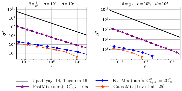
Randomized sketching is a central tool for compressing large-scale optimization problems while preserving accuracy. In particular, sketches that are based on structured matrices, such as the Hadamard matrix, can be applied efficiently and often yield solutions that approximate those of the original problem at much lower computational cost. In differential privacy (DP), Gaussian sketching has been used to solve DP linear regression, beginning with \citet{sheffet2017differentially, sheffet2019old} and later refined by \citet{lev2025gaussianmix, lev2026near}. However, although these methods achieve strong utility guarantees, they usually do not improve runtime over classical DP approaches. In this work, we introduce a new DP sketching mechanism based on fast transforms, which, in certain cases, matches the runtime of classical fast sketching methods. We prove state-of-the-art privacy guarantees for this mechanism and show that, in favorable regimes, they match those of the Gaussian sketch up to a constant factor. As an application, we combine this mechanism with recent sketch-based methods for DP linear regression to obtain a new algorithm with strong utility and improved runtime. We establish privacy and accuracy guarantees for this algorithm, yielding, to the best of our knowledge, the first fast method for DP ordinary least squares.
Editorial analysis
A structured set of objections, weighed in public.
Referee Report
Summary. The paper introduces a fast mixing mechanism for differential privacy based on structured fast transforms (e.g., randomized Hadamard), proves state-of-the-art privacy guarantees for the mechanism, shows that these guarantees match those of the Gaussian sketch up to a constant factor in favorable regimes, and applies the mechanism to obtain the first fast algorithm for DP ordinary least squares with matching utility.
Significance. If the central claims hold, the work would be significant for large-scale DP optimization: it combines the runtime benefits of classical fast sketching with DP guarantees that avoid the slowdown of Gaussian methods, while delivering the first fast DP OLS solver. The explicit re-derivation of privacy and utility bounds from the properties of fast transforms (rather than black-box transfer) would be a notable technical contribution.
major comments (1)
- [Privacy analysis of the fast mixing mechanism] The privacy analysis for the fast mixing mechanism (main theorem on privacy guarantees): the claim that the mechanism matches Gaussian-sketch privacy up to a constant factor requires an explicit first-principles derivation of the relevant sub-Gaussian tail bounds and sensitivity for the structured fast transform; if the proof invokes rotational invariance or concentration lemmas that hold only for i.i.d. Gaussian entries without re-deriving the failure probabilities or log factors for the fast case, the constant-factor statement does not hold outside narrow parameter regimes.
minor comments (2)
- [Abstract and §1] The abstract and introduction repeatedly use the qualifiers 'in certain cases' and 'favorable regimes' without stating the precise conditions on sketch size, dimension, or failure probability; these should be stated explicitly (e.g., as a displayed assumption or theorem statement) so readers can assess applicability.
- [Preliminaries] Notation for the fast transform matrix and the mixing parameter should be introduced once with a clear definition before the first use in the privacy proof, to avoid ambiguity when comparing to the Gaussian case.
Simulated Author's Rebuttal
We thank the referee for their thoughtful review and for highlighting the importance of a rigorous first-principles privacy analysis. We address the single major comment below.
read point-by-point responses
-
Referee: [Privacy analysis of the fast mixing mechanism] The privacy analysis for the fast mixing mechanism (main theorem on privacy guarantees): the claim that the mechanism matches Gaussian-sketch privacy up to a constant factor requires an explicit first-principles derivation of the relevant sub-Gaussian tail bounds and sensitivity for the structured fast transform; if the proof invokes rotational invariance or concentration lemmas that hold only for i.i.d. Gaussian entries without re-deriving the failure probabilities or log factors for the fast case, the constant-factor statement does not hold outside narrow parameter regimes.
Authors: We agree that a first-principles derivation is essential and believe the manuscript already supplies one. In the proof of the main privacy theorem (Theorem 3.2), we derive the sub-Gaussian norm and tail bounds directly from the mixing properties of the fast structured transform (randomized Hadamard followed by the mixing matrix) and the coordinate-wise sensitivity of the sketch. The argument uses only the known concentration of the fast transform (via its recursive structure and union bounds over the Walsh basis) together with a direct calculation of the privacy loss random variable; it does not invoke rotational invariance of Gaussians or any Gaussian-specific lemmas. The resulting failure probabilities and logarithmic factors are tracked explicitly and appear in the final constant-factor comparison (see the regime statements in Theorem 3.2 and the discussion following Corollary 3.3). We are therefore confident that the constant-factor claim holds in the stated favorable regimes. If the referee can point to a specific step that appears to rely on an un-rederived Gaussian fact, we will gladly expand that step in the revision. revision: no
Circularity Check
No circularity; new mechanism's privacy analysis presented as independent
full rationale
The abstract and context describe introduction of a new fast-transform DP sketching mechanism with claimed proofs of privacy guarantees that match Gaussian sketches up to constant factor in favorable regimes, plus an application to DP OLS. No equations, fitted parameters, or derivations are shown reducing by construction to inputs, self-citations, or ansatzes. Self-citations to Lev et al. (2025/2026) supply background on prior Gaussian work but are not invoked as the sole justification for the new mechanism's bounds; the paper states it proves the new guarantees separately. This matches the default expectation of a self-contained derivation with no load-bearing reduction to prior self-work.
Axiom & Free-Parameter Ledger
invented entities (1)
-
Fast mixing mechanism
no independent evidence
Reference graph
Works this paper leans on
-
[1]
A History of Census Privacy Protections
United States Census Bureau. A History of Census Privacy Protections. https://www.census. gov/library/visualizations/2019/comm/history-privacy-protection.html,
2019
-
[2]
Manuel Gil, Fady Alajaji, and Tamas Linder
URL https://research.facebook.com/blog/2020/6/ protecting-privacy-in-facebook-mobility-data-during-the-covid-19-response/. Manuel Gil, Fady Alajaji, and Tamas Linder. R´ enyi divergence measures for commonly used univariate continuous distributions.Information Sciences, 249:124–131,
2020
-
[3]
Tamas Sarlos
Accessed: 2022-07-28. Tamas Sarlos. Improved approximation algorithms for large matrices via random projections. In 2006 47th annual IEEE symposium on foundations of computer science, pages 143–152. IEEE,
2022
-
[4]
Jalaj Upadhyay. Randomness-efficient fast Johnson–Lindenstrauss transform with applications in differential privacy and compressed sensing.arXiv preprint arXiv:1410.2470,
work page internal anchor Pith review Pith/arXiv arXiv
-
[5]
We will first provide a proof of Lemma
C Proof of Theorem 1 Our proof will use the next standard formula for the R´ enyi divergence between two d-dimensional multivariate Gaussian distributions [Gil et al., 2013] Dα N ⃗0d,Σ 1 N ⃗0d,Σ 2 =− 1 2(α−1) log det (Σ1 +α(Σ 2 −Σ 1)) (det (Σ1))1−α (det (Σ2))α (6) which holds for allαsuch thatαΣ −1 1 + (1−α)Σ −1 2 = Σ−1 2 +α Σ−1 1 −Σ −1 2 ≻0. We will firs...
2013
-
[6]
[2025, Corollary
Thus, using Lev et al. [2025, Corollary. 1], we know that this is upper bounded by 1 2(α−1) α·log 1− 5 4γ −log 1− 5α 4γ ≤ 25α 32γ2 for all α∈ (1, 8γ/25) and provided that γ≥ 25/8. This establishes the bound presented in Lemma
2025
-
[7]
whenever S⊤ f Sf = In. In this case, we getC 2 Sf X = 1, and the overall divergence becomes 1 2(α−1) α·log 1− 1 λX min +σ 2 −log 1− α λX min +σ 2 and for λX min+σ2 > 1 and 1 < α < λ X min+σ2, which recovers exactly the analysis from Lev et al. [2025, Appendix. B]. We note that in this case, Sf is an orthogonal matrix, sog ⊤Sf ∼N (⃗0n,I n), which is distri...
2025
-
[8]
Lemma 3.Letu, v∈R d
Throughout, we use the notion of ℓ1 sensitivity, which, given a target functionf(X), is defined by max (X,X ′):X ′≃X f(X)−f(X ′) . Lemma 3.Letu, v∈R d. Then, uv⊤ op =∥u∥ ∥v∥, uv⊤ +vu ⊤ op =∥u∥ ∥v∥+ u⊤v . Proof. If either u = ⃗0d or v = ⃗0d, both identities are immediate. Hence, assume u, v̸ = ⃗0d, and define u := u ∥u∥ , v := v ∥v∥ . We first calculate th...
1991
-
[9]
First, note that for the τ stated in the theorem and by using a union-bound, it holds P(E c)≤P bλ≤ eλ +P(em≤bm) =P(z 1 ≥τ) +P(z 2 ≥τ)≤ 2δ 3
o wherez 1 ∼Lap(0,1) eλ max n 0, λSf X min −ω(bΛ + 2em)(τ−z2) o wherez 2 ∼Lap(0,1) Let E := n eλ≤bλ T(em≥bm) o . First, note that for the τ stated in the theorem and by using a union-bound, it holds P(E c)≤P bλ≤ eλ +P(em≤bm) =P(z 1 ≥τ) +P(z 2 ≥τ)≤ 2δ 3 . From now on, we prove the privacy guarantees of the mechanism conditioned on the event E, where by Lem...
2014
-
[10]
Computing Z.Involves applying an SRHT of size ( k2, n) to X∈R n×d
C.4.2 Runtime Complexity We provide the proof by explicitly writing the complexity of the different steps inside FastMix and their runtime complexity. Computing Z.Involves applying an SRHT of size ( k2, n) to X∈R n×d. Following classical arguments (see, for example, Ailon and Liberty [2009]), the runtime complexity of this step is O(ndlog (k2)). However, ...
2009
-
[11]
Therefore, U ⊤ S⊤ HSH −I n ei = R⊤ i Q⊤ i S⊤ HSH −I n Qiqi ≤ Q⊤ i S⊤ HSH −I n Qi op
Since both U and ei belong to span(Qi), there existR i andq i such that U=Q iRi, e i =Q iqi,∥R i∥op ≤1,∥q i∥2 ≤1. Therefore, U ⊤ S⊤ HSH −I n ei = R⊤ i Q⊤ i S⊤ HSH −I n Qiqi ≤ Q⊤ i S⊤ HSH −I n Qi op . Hence X ⊤ S⊤ HSH −I n ei ≤ ∥X∥ op Q⊤ i S⊤ HSH −I n Qi op . Then, for each fixedi, by Cohen et al. [2016, Theorem. 9] it holds that E Q⊤ i S⊤ HSH −I n Qi 2 op...
2016
-
[12]
By Markov’s inequality, this further implies that P Q⊤ i S⊤ HSH −I n Qi op > χ ≤δ i
+ log 1 χδi log r+ 1 δi for a universal constantC >0. By Markov’s inequality, this further implies that P Q⊤ i S⊤ HSH −I n Qi op > χ ≤δ i. Consequently, P X ⊤ S⊤ HSH −I n ei > χ∥X∥ op ≤δ i. Then, choosingδ i := ϱ/nand union bounding overi∈[n] yields P max i∈[n] X ⊤ S⊤ HSH −I n ei > χ∥X∥ op ≤ nX i=1 δi =ϱ. This completes the proof. Lemma 10.Let X∈R n×d and...
2016
-
[13]
Throughout, quantities computed in the t’th call toFastMixare indexed byt for example,emt,eλt,S H,t,S G,t . Our proof uses Lemma 7 and Lemma 1 to calculate the RDP guarantees for each step forming eGt and eXt, and then applies the RDP composition theorem to obtain their overall guarantees separately. In particular, we separate the contribution of the Lapl...
2020
-
[14]
and seek to obtain an high probability bound on ∥bθT −θ ∗∥2 X ⊤X, which corresponds to the excess empirical risk [Wang, 2018, Lemma. 5]. Recall that in terms of notation, emt denote the private version of bmt andeλt the private version ofbλt, wherebλt :=λ SH,tX min .For anya≥0, we define X a := (X ⊤, aI d)⊤ andM a :=X ⊤X+a 2Id = X ⊤ a X a. Step 1: Definin...
2018
-
[15]
We note that the eventB tot(χ) implies λSH,tX min ≥(1−χ)λ X min and max i∈[n] X ⊤ S⊤ H,tSH,t −I n ei ≤ χ 2 ∥X∥op for allt= 0, . . . , T−1. This holds since for everyi∈[n], the eventB 2,t(χ) implies X ⊤ S⊤ H,tSH,t −I n ei = sup ∥v∥=1 e⊤ i S⊤ H,tSH,t −I n Xv ≤ χ 2 sup ∥v∥=1 ∥Xv∥= χ 2 ∥X∥op . Conditioning onB tot(χ), we next define for eacht= 0, . . . , T−1 ...
2016
-
[16]
[2026, Appendix
As in Lev et al. [2026, Appendix. C], for χ below a sufficiently small constant less than 1 4, attainable by increasing k1 and k2 by constant factors, this bound is less than C whenever C≥a 0 ·max{C Y ,∥θ ∗∥} and k1 ≥a 1 ·κ X(η2)·d, k 2 ≥a 1 ·κ X(η2)·d·log 4(n) for constantsa 0, a1. Now, to further simplify this argument, we note that κX η2 = λX max −λ X ...
2026
-
[17]
we get that the constraints onk 1, k2 can be enforced by setting k1 ≥a 2 · d· λX max −λ X min εp log(1/δ) !2/3 , k 2 ≥a 2 · d· λX max −λ X min εp log(1/δ) ·log 4(n) !2/3 . Overall, conditioned onA tot clipping does not occur provided thatC≥a 0 ·max{C Y ,∥θ ∗∥}and k1χ2 ≥a 2 ·max d, gX ,log 8T¯cG ϱ , √ 2d+ p 4 log (8T/ϱ) 2 , k2χ2 ≥a 2 ·max ( rank(X) log4(n)...
2026
-
[18]
[2021, Section 4.1]), b∆≥ s n−k k(n−1)
Moreover, by Welch’s lower bound [Welch, 1974, Theorem 1] (see also the discussion in Haikin et al. [2021, Section 4.1]), b∆≥ s n−k k(n−1) . In particular, when n k ≫ 1, the optimal coherence scale permitted by Welch’s bound is Θ k−1/2 , while for n≈k + 1 it might get as small as Θ k−1 . For the SRHT, as shown in Appendix E, w.p. at least 1−ϱthere exists ...
1974
-
[19]
For performing the Hadamard transform, we have used the optimized implementation from https://github.com/falconn-lib/ffht
The airline dataset was subsampled to 4194304 points, to allow for reasonable solution times. For performing the Hadamard transform, we have used the optimized implementation from https://github.com/falconn-lib/ffht. We report the excess empirical risk. First, we calculate the normalized mean squared error (MSE) for the train set, computed as the squared ...
2026
-
[20]
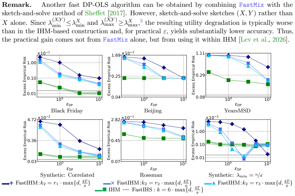
For both schemes, we omitted the term −η2bθt from the computation of eGt, as it improves performance by making the iterates converge closer to θ∗ than to θ∗(η2)
For FastIHM, we used k1 = 6 ·max{d,log( 4T/ϱ)}, T = 4 and C = CY . For both schemes, we omitted the term −η2bθt from the computation of eGt, as it improves performance by making the iterates converge closer to θ∗ than to θ∗(η2). This does not affect the privacy analysis, so we omit this term in the empirical evaluation. Whenever we used the Gaussian mecha...
2018
-
[21]
and σ2 = 0 .1. The second dataset aims to test the performance of the algorithm in a poorly conditioned setting (termedsynthetic correlated), where usually the computational advantage of the IHS becomes prominent (see, for example, experiments done in Pilanci and Wainwright [2016], Lacotte et al. [2020]). To that end, we generate a design matrix built fro...
2016
-
[22]
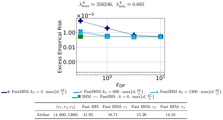
In particular, we use the airline dataset [ope, 2020], subsampled to n = 222 samples, leads to n/d = 222 /4 =
I Additional Experiments We now provide additional experiments for a setting where the ratio n/d is extremely large, rep- resenting a setting where sketching is most beneficial in terms of runtime. In particular, we use the airline dataset [ope, 2020], subsampled to n = 222 samples, leads to n/d = 222 /4 =
2020
-
[23]
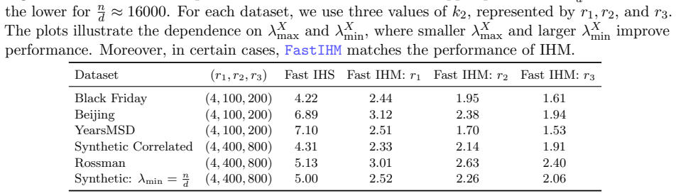
We sweep across values of k2 max{d,log(4T/ϱ)} ∈ [4, 1200] and fix T = 4 , k1 = 6 ·max{d,log( 4T/ϱ)} and k = 6 ·max{d,log( 4T/ϱ)}. As seen in Figure 4, in this regime, FastIHM allows for attaining close-to- optimal performance at a significantly lower runtime, demonstrating the most favorable regime for sketching. J Dataset Statistics The next table summar...
2018
discussion (0)
Sign in with ORCID, Apple, or X to comment. Anyone can read and Pith papers without signing in.