Radio Continuum Emission from Evolving Star-Forming Galaxies -- I. Correlations Involving the Total Synchrotron Luminosity
Pith reviewed 2026-06-28 14:07 UTC · model grok-4.3
The pith
Models show synchrotron luminosity from star-forming galaxies correlates strongly with both star formation rate and rotation speed out to redshift 3.
A machine-rendered reading of the paper's core claim, the machinery that carries it, and where it could break.
Core claim
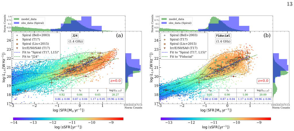
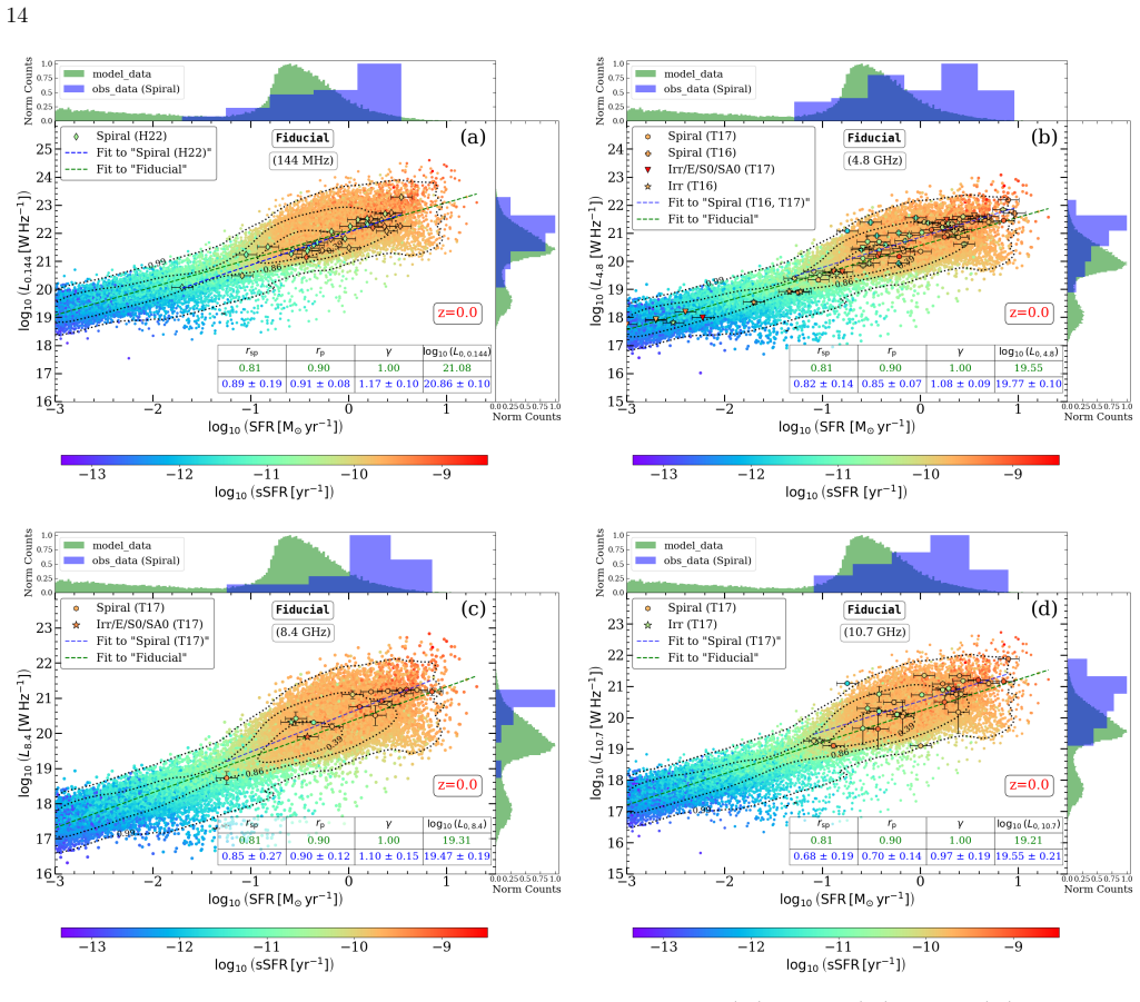
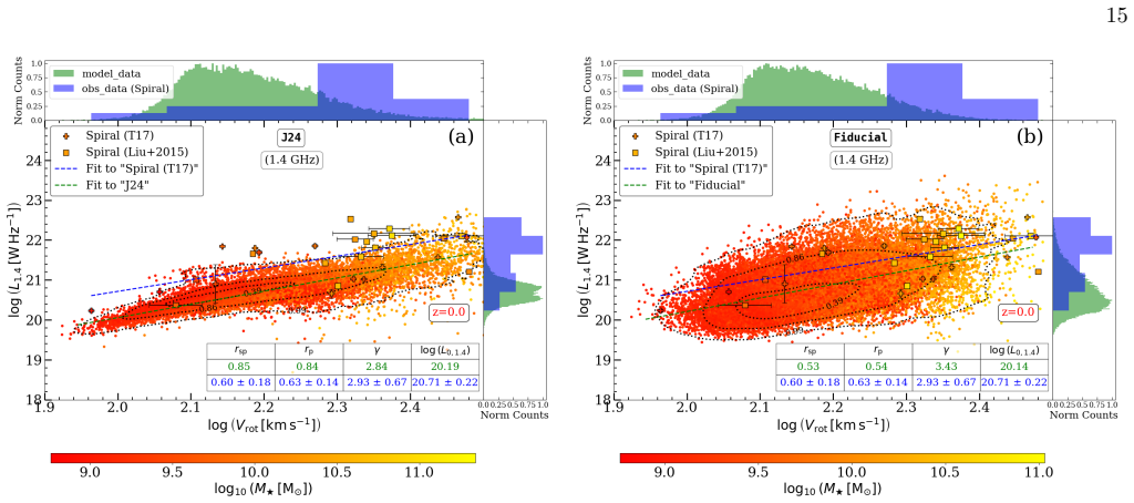
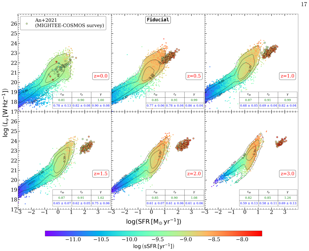
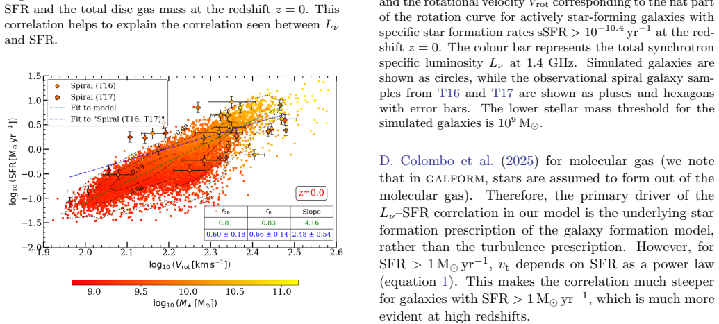
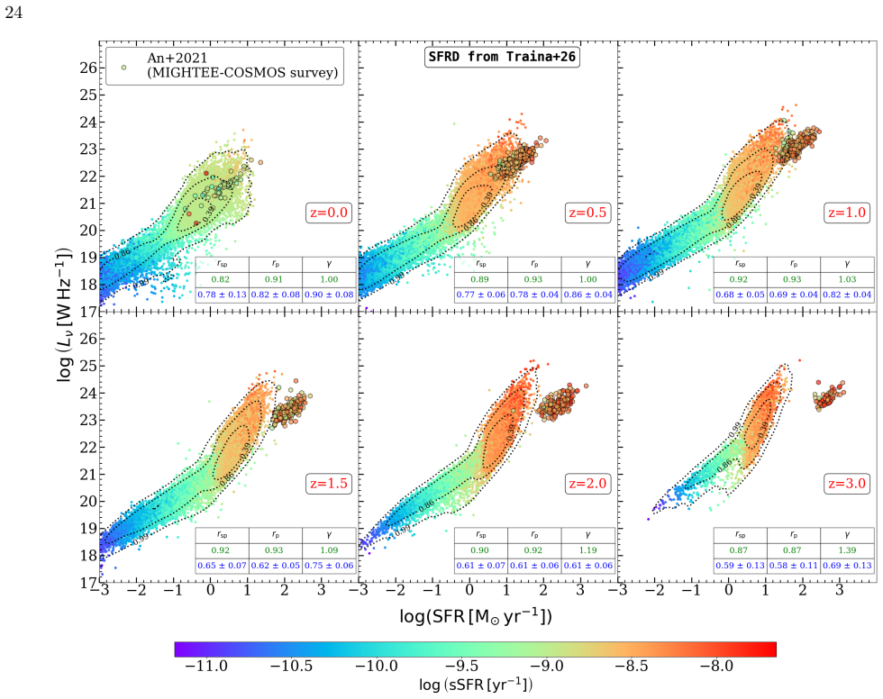
Strong positive correlations exist between the specific synchrotron luminosity L_ν and both the star formation rate SFR and the characteristic galaxy rotation speed V_rot for redshifts up to z ≃ 3. These correlations arise from the tight link between disc gas mass and SFR together with the stellar-mass Tully-Fisher relation. At low redshifts the turbulent magnetic field dominates the luminosity, while the contribution of the large-scale field increases with redshift and becomes important for z ≳ 1. The models agree with compiled observational data at low redshift but under-predict SFR at higher redshift.
What carries the argument
The combination of the GALFORM semi-analytic galaxy formation model with the MAGNETIZER dynamo code, used to compute synchrotron luminosity under local cosmic-ray–magnetic-field equipartition.
If this is right
- The correlation between L_ν and SFR follows directly from the correlation between disc gas mass and SFR.
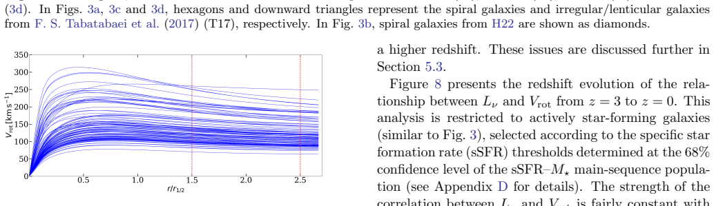
- The additional correlation between L_ν and V_rot follows from the stellar-mass Tully–Fisher relation obeyed by main-sequence galaxies.
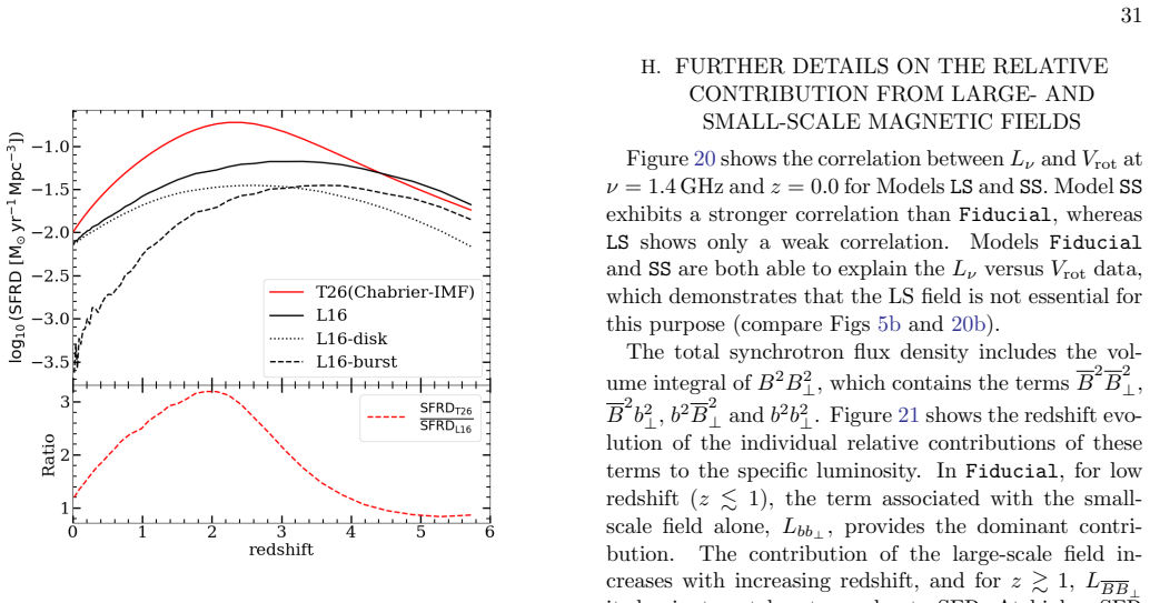
- Turbulent magnetic fields dominate the synchrotron luminosity at low redshift while the large-scale field contribution rises and becomes significant for z ≳ 1.
- Model predictions match existing radio data at low redshift but yield systematically smaller SFR values than earlier observational estimates at higher redshift.
Where Pith is reading between the lines
- If the correlations hold, total radio luminosity could serve as a dust-independent proxy for star-formation rate once the high-redshift discrepancy is resolved.
- The growing importance of the ordered field with redshift implies that polarization surveys at z > 1 will increasingly trace large-scale galactic dynamos rather than turbulence alone.
- The same scaling relations could be inverted to estimate rotation speeds of distant galaxies from radio continuum maps alone, providing an independent check on the Tully–Fisher relation.
Load-bearing premise
Local energy equipartition between cosmic rays and magnetic fields is assumed when converting simulated magnetic-field strengths into synchrotron luminosity.
What would settle it
A set of radio observations at z > 1 that shows no correlation between total synchrotron luminosity and either SFR or V_rot would falsify the reported relations.
Figures


read the original abstract
Synchrotron radiation dominates the continuum emission of star-forming galaxies in the frequency range from a few $\rm MHz$ to about $30\,\rm{GHz}$. We model the total synchrotron emission of a large population of evolving star-forming galaxies using the semi-analytic galaxy formation model GALFORM combined with the dynamo simulation code MAGNETIZER. Assuming local energy equipartition between cosmic rays and magnetic fields, we calculate the specific synchrotron luminosity $L_{\nu}$ for each simulated galaxy at various frequencies and find strong positive correlations between $L_{\nu}$ and both the star formation rate ($\rm SFR$) and characteristic galaxy rotation speed $V_{\rm rot}$ for redshifts up to $z\simeq 3$. At low redshifts, the turbulent magnetic field is found to dominate in the synchrotron luminosity, but the contribution of the large-scale magnetic field increases with redshift and becomes important for $z\gtrsim 1$. The correlation between $L_{\nu}$ and $\rm SFR$ arises from the tight correlation between the disc gas mass $M_{\rm gas}$ and $\rm SFR$, and the correlation between $L_{\nu}$ and $V_{\rm rot}$ is additionally a consequence of the stellar mass Tully--Fisher relation for main-sequence galaxies. At low redshifts, the model predictions and observational data compiled for this work show remarkable agreement, but a discrepancy arises at higher redshifts, where modelled $\rm SFR$ values are systematically smaller than those previously inferred from observations. These theoretical models will aid the interpretation of next-generation radio surveys with the Square Kilometre Array and other telescopes.
Editorial analysis
A structured set of objections, weighed in public.
Referee Report
Summary. The manuscript couples the GALFORM semi-analytic galaxy formation model with the MAGNETIZER dynamo code to compute the total synchrotron luminosity L_ν of a population of evolving star-forming galaxies. Under the explicit assumption of local energy equipartition between cosmic rays and magnetic fields, it reports strong positive correlations between L_ν and both SFR and V_rot up to z ≃ 3. Turbulent fields dominate the luminosity at low z while the large-scale field contribution grows and becomes important for z ≳ 1. The correlations are traced to the M_gas–SFR relation and the stellar-mass Tully–Fisher relation. Model–observation agreement is described as remarkable at low z, but the model systematically underpredicts SFR at higher redshifts.
Significance. If the equipartition assumption remains valid, the work supplies a physically motivated framework for predicting radio continuum emission that can be used to interpret SKA and other next-generation surveys. The separation of turbulent versus large-scale field contributions and the explicit linkage of the correlations to established galaxy scaling relations are clear strengths. The absence of quantitative error bars, independent validation data sets, and tests of the equipartition assumption at z > 1 nevertheless restricts the immediate utility of the reported relations.
major comments (2)
- [Abstract and §2] Abstract and §2 (model description): L_ν is obtained solely by imposing local equipartition on the B-field and CR energy densities output by MAGNETIZER. No sensitivity run is shown in which the equipartition ratio is allowed to vary with redshift or with the increasing large-scale-field fraction at z ≳ 1; such a variation would directly rescale the derived L_ν values and therefore alter the slopes and scatter of the L_ν–SFR and L_ν–V_rot relations that constitute the central claim.
- [§4] §4 (high-redshift comparison): The text notes that modelled SFR values lie systematically below observational inferences at z > 1. Because L_ν is computed from the same gas and magnetic-field quantities that also set the SFR, any additional systematic shift arising from a redshift-dependent departure from equipartition would compound the existing discrepancy and weaken the assertion that the correlations can be applied to interpret SKA observations at z > 1.
minor comments (1)
- [Abstract] Abstract: the phrase 'remarkable agreement' at low redshifts is not accompanied by any quantitative metric (e.g., reduced χ², median offset, or scatter) that would allow the reader to judge the level of agreement.
Simulated Author's Rebuttal
We thank the referee for their constructive and detailed report. We address each major comment below, providing our responses and indicating whether revisions will be made.
read point-by-point responses
-
Referee: [Abstract and §2] Abstract and §2 (model description): L_ν is obtained solely by imposing local equipartition on the B-field and CR energy densities output by MAGNETIZER. No sensitivity run is shown in which the equipartition ratio is allowed to vary with redshift or with the increasing large-scale-field fraction at z ≳ 1; such a variation would directly rescale the derived L_ν values and therefore alter the slopes and scatter of the L_ν–SFR and L_ν–V_rot relations that constitute the central claim.
Authors: The manuscript explicitly adopts local energy equipartition as a standard and well-motivated assumption for calculating synchrotron luminosity from the magnetic field and cosmic-ray energy densities provided by MAGNETIZER. The reported correlations are derived and presented under this assumption. There is currently no consensus or physically motivated prescription for how the equipartition ratio might vary with redshift or with the relative contribution of the large-scale field; introducing arbitrary variations would therefore add unconstrained parameters without improving the physical interpretation. We have revised Section 2 to state more explicitly that all quantitative results are conditional on the equipartition assumption and have added a brief discussion of this limitation in the conclusions. revision: partial
-
Referee: [§4] §4 (high-redshift comparison): The text notes that modelled SFR values lie systematically below observational inferences at z > 1. Because L_ν is computed from the same gas and magnetic-field quantities that also set the SFR, any additional systematic shift arising from a redshift-dependent departure from equipartition would compound the existing discrepancy and weaken the assertion that the correlations can be applied to interpret SKA observations at z > 1.
Authors: The systematic underprediction of SFR at z > 1 is already noted in the manuscript and arises from the underlying GALFORM model. Because L_ν is computed self-consistently from the same gas mass and magnetic-field quantities that determine the SFR within the model, the L_ν–SFR and L_ν–V_rot relations remain internally consistent under the maintained equipartition assumption. We agree that any unmodeled redshift dependence in the equipartition ratio would affect the absolute normalization at high z. We have expanded the discussion in Section 4 to caution that the reported correlations should be applied to SKA data at z ≳ 1 only with this caveat in mind. revision: partial
Circularity Check
No significant circularity; correlations are model outputs from external codes under stated assumption
full rationale
The paper runs established external codes (GALFORM, MAGNETIZER) to generate galaxy populations, then computes L_ν from simulated B and CR densities under the explicit local equipartition assumption. The reported L_ν–SFR and L_ν–V_rot correlations are shown to follow directly from the model's pre-existing M_gas–SFR relation and the stellar-mass Tully–Fisher relation; neither correlation is fitted to the target data nor defined in terms of itself. No self-citation is invoked as a uniqueness theorem or load-bearing premise, and no parameter is tuned on a subset of the reported relations and then relabeled a prediction. The high-z discrepancy with observed SFR is noted openly rather than adjusted away. The derivation chain is therefore self-contained against external benchmarks.
Axiom & Free-Parameter Ledger
axioms (1)
- domain assumption local energy equipartition between cosmic rays and magnetic fields
Reference graph
Works this paper leans on
-
[1]
2021, MNRAS, 507, 2643, doi: 10.1093/mnras/stab2290
An, F., Vaccari, M., Smail, I., et al. 2021, MNRAS, 507, 2643, doi: 10.1093/mnras/stab2290
-
[2]
2016, A&A, 587, A86, doi: 10.1051/0004-6361/201527812
Baes, M., & Viaene, S. 2016, A&A, 587, A86, doi: 10.1051/0004-6361/201527812
-
[3]
Baugh, C. M., Lacey, C. G., Frenk, C. S., et al. 2005, MNRAS, 356, 1191, doi: 10.1111/j.1365-2966.2004.08553.x
-
[4]
2015, ARA&A, 24, 4, doi: 10.1007/s00159-015-0084-4
Beck, R. 2015, ARA&A, 24, 4, doi: 10.1007/s00159-015-0084-4
-
[5]
1996, ARA&A, 34, 155, doi: 10.1146/annurev.astro.34.1.155
Sokoloff, D. 1996, ARA&A, 34, 155, doi: 10.1146/annurev.astro.34.1.155
-
[6]
Beck, R., Chamandy, L., Elson, E., & Blackman, E. G. 2019, Galaxies, 8, 4, doi: 10.3390/galaxies8010004
-
[7]
2005, Astronomische Nachrichten, 326, 414, doi: 10.1002/asna.200510366
Beck, R., & Krause, M. 2005, Astronomische Nachrichten, 326, 414, doi: 10.1002/asna.200510366
-
[8]
D., Shukurov, A., & Sokoloff, D
Beck, R., Poezd, A. D., Shukurov, A., & Sokoloff, D. D. 1994, A&A, 289, 94
1994
-
[9]
Beck, R., & Wielebinski, R. 2013, in Planets, Stars and Stellar Systems. Volume 5: Galactic Structure and Stellar Populations, ed. T. D. Oswalt & G. Gilmore (Springer Netherlands), 641, doi: 10.1007/978-94-007-5612-0 13
-
[10]
2026, A&A, 707, A396, doi: 10.1051/0004-6361/202557901
Paladino, R. 2026, A&A, 707, A396, doi: 10.1051/0004-6361/202557901
-
[11]
Bell, E. F. 2003, ApJ, 586, 794, doi: 10.1086/367829
-
[12]
2020, ApJ, 903, 10, doi: 10.3847/1538-4357/abb5f4 32 Figure 20.Similar to Fig
Belland, B., Kirby, E., Boylan-Kolchin, M., & Wheeler, C. 2020, ApJ, 903, 10, doi: 10.3847/1538-4357/abb5f4 32 Figure 20.Similar to Fig. 5b, but with contribution of large-scale ( B) (panel 20a) and small-scale (b) (panel 20b) field only. Figure 21.The redshift evolution of the ratios of the specific luminosities contributed by different terms —-b 2b⊥2, B...
-
[13]
2020, A&A, 634, A124, doi: 10.1051/0004-6361/201937284
Bellazzini, M., Annibali, F., Tosi, M., et al. 2020, A&A, 634, A124, doi: 10.1051/0004-6361/201937284
-
[14]
Besla, G., Kallivayalil, N., Hernquist, L., et al. 2012, MNRAS, 421, 2109, doi: 10.1111/j.1365-2966.2012.20466.x
-
[15]
Best, P. N., Kauffmann, G., Heckman, T. M., & Ivezi´ c,ˇZ. 2005, MNRAS, 362, 9, doi: 10.1111/j.1365-2966.2005.09283.x
-
[16]
2004, ApJ, 612, L29, doi: 10.1086/424661
Blitz, L., & Rosolowsky, E. 2004, ApJ, 612, L29, doi: 10.1086/424661
-
[17]
2006, ApJ, 650, 933, doi: 10.1086/505417
Blitz, L., & Rosolowsky, E. 2006, ApJ, 650, 933, doi: 10.1086/505417
-
[18]
Bogue, K. R. J., Smith, R. J., Treß, R. G., et al. 2026, MNRAS, 545, staf2132, doi: 10.1093/mnras/staf2132
-
[19]
2003, in Advances in Nonlinear Dynamics (London: Taylor & Francis), 269
Brandenburg, A. 2003, in Advances in Nonlinear Dynamics (London: Taylor & Francis), 269
2003
-
[20]
2005, PhR, 417, 1, doi: 10.1016/j.physrep.2005.06.005
Brandenburg, A., & Subramanian, K. 2005, PhR, 417, 1, doi: 10.1016/j.physrep.2005.06.005
-
[21]
2003, PASP, 115, 763, doi: 10.1086/376392
Chabrier, G. 2003, PASP, 115, 763, doi: 10.1086/376392
work page internal anchor Pith review doi:10.1086/376392 2003
-
[22]
2016, MNRAS, 462, 4402, doi: 10.1093/mnras/stw1941
Chamandy, L. 2016, MNRAS, 462, 4402, doi: 10.1093/mnras/stw1941
-
[23]
Chamandy, L., Nazareth, R. G., & Santhosh, G. 2024, ApJ, 966, 78, doi: 10.3847/1538-4357/ad3205
-
[24]
2020, Galaxies, 8, 56, doi: 10.3390/galaxies8030056
Chamandy, L., & Shukurov, A. 2020, Galaxies, 8, 56, doi: 10.3390/galaxies8030056
-
[25]
2014, MNRAS, 443, 1867, doi: 10.1093/mnras/stu1274
Chamandy, L., Shukurov, A., Subramanian, K., & Stoker, K. 2014, MNRAS, 443, 1867, doi: 10.1093/mnras/stu1274
-
[26]
Chamandy, L., Shukurov, A., & Taylor, A. R. 2016, ApJ, 833, 43, doi: 10.3847/1538-4357/833/1/43
-
[27]
Chamandy, L., & Taylor, A. R. 2015, ApJ, 808, 28, doi: 10.1088/0004-637X/808/1/28
-
[28]
S., Ruszkowski, M., Werhahn, M., Pfrommer, C., & Thomas, T
Chiu, H.-H. S., Ruszkowski, M., Werhahn, M., Pfrommer, C., & Thomas, T. 2025, arXiv e-prints, arXiv:2510.03229, doi: 10.48550/arXiv.2510.03229 Chy˙ zy, K. T., Sridhar, S. S., & Jurusik, W. 2017, A&A, 603, A121, doi: 10.1051/0004-6361/201730690 Chy˙ zy, K. T., We˙ zgowiec, M., Beck, R., & Bomans, D. J. 2011, A&A, 529, A94, doi: 10.1051/0004-6361/201015393
-
[29]
Cole, S., Lacey, C. G., Baugh, C. M., & Frenk, C. S. 2000, MNRAS, 319, 168, doi: 10.1046/j.1365-8711.2000.03879.x
-
[30]
2025, A&A, 699, A367, doi: 10.1051/0004-6361/202453217
Colombo, D., Kalinova, V., Bazzi, Z., et al. 2025, A&A, 699, A367, doi: 10.1051/0004-6361/202453217
-
[31]
Condon, J. J., Cotton, W. D., & Broderick, J. J. 2002, AJ, 124, 675, doi: 10.1086/341650
-
[32]
Condon, J. J., Matthews, A. M., & Broderick, J. J. 2019, ApJ, 872, 148, doi: 10.3847/1538-4357/ab0301
-
[33]
2014, A&A, 572, A23, doi: 10.1051/0004-6361/201424033
Salucci, P. 2014, A&A, 572, A23, doi: 10.1051/0004-6361/201424033
-
[34]
2024, MNRAS, 527, 10358, doi: 10.1093/mnras/stad3892
Das, S., Rickel, M., Leroy, A., et al. 2024, MNRAS, 527, 10358, doi: 10.1093/mnras/stad3892
-
[35]
Erkal, D., Belokurov, V., Laporte, C. F. P., et al. 2019, MNRAS, 487, 2685, doi: 10.1093/mnras/stz1371
-
[36]
Bushby, P. J. 2019, MNRAS, 488, 5065, doi: 10.1093/mnras/stz2084
-
[37]
2011, PhRvL, 107, 114504, doi: 10.1103/PhysRevLett.107.114504
Federrath, C., Chabrier, G., Schober, J., et al. 2011, PhRvL, 107, 114504, doi: 10.1103/PhysRevLett.107.114504
-
[38]
2020, Communications Physics, 3, 226, doi: 10.1038/s42005-020-00493-0
Feldmann, R. 2020, Communications Physics, 3, 226, doi: 10.1038/s42005-020-00493-0
-
[39]
2017, ApJ, 841, 51, doi: 10.3847/1538-4357/aa6d63
Foord, A., Gallo, E., Hodges-Kluck, E., et al. 2017, ApJ, 841, 51, doi: 10.3847/1538-4357/aa6d63
-
[40]
Garn, T., Green, D. A., Riley, J. M., & Alexander, P. 2009, MNRAS, 397, 1101, doi: 10.1111/j.1365-2966.2009.15073.x
-
[41]
A., Mac Low, M.-M., & Korpi-Lagg, M
Gent, F. A., Mac Low, M.-M., & Korpi-Lagg, M. J. 2024, ApJ, 961, 7, doi: 10.3847/1538-4357/ad0da0
-
[42]
2022, ApJ, 932, 44, doi: 10.3847/1538-4357/ac6750
Gilhuly, C., Merritt, A., Abraham, R., et al. 2022, ApJ, 932, 44, doi: 10.3847/1538-4357/ac6750
-
[43]
2023, ApJ, 943, 66, doi: 10.3847/1538-4357/aca808
Gopalakrishnan, K., & Subramanian, K. 2023, ApJ, 943, 66, doi: 10.3847/1538-4357/aca808
-
[44]
2023, MNRAS, 520, 4902, doi: 10.1093/mnras/stad114
Groves, B., Kreckel, K., Santoro, F., et al. 2023, MNRAS, 520, 4902, doi: 10.1093/mnras/stad114
-
[45]
Guo, Q., White, S., Angulo, R. E., et al. 2013, MNRAS, 428, 1351, doi: 10.1093/mnras/sts115
-
[46]
Hansen, S. P., Lagos, C. D. P., Bonato, M., et al. 2024, MNRAS, 531, 1971, doi: 10.1093/mnras/stae1235
-
[47]
Harmsen, B., Monachesi, A., Bell, E. F., et al. 2017, MNRAS, 466, 1491, doi: 10.1093/mnras/stw2992
-
[48]
Heald, G. H., Heesen, V., Sridhar, S. S., et al. 2022, MNRAS, 509, 658, doi: 10.1093/mnras/stab2804
-
[49]
2022, A&A, 664, A83, doi: 10.1051/0004-6361/202142878
Heesen, V., Staffehl, M., Basu, A., et al. 2022, A&A, 664, A83, doi: 10.1051/0004-6361/202142878
-
[50]
1990, ApJ, 356, 359, doi: 10.1086/168845
Hernquist, L. 1990, ApJ, 356, 359, doi: 10.1086/168845
-
[51]
Gent, F. A. 2017, ApJ, 850, 4, doi: 10.3847/1538-4357/aa93e7
-
[52]
Hopkins, A. M., & Beacom, J. F. 2006, ApJ, 651, 142, doi: 10.1086/506610
-
[53]
Hosseinirad, M., Tabatabaei, F., Raouf, M., & Roshan, M. 2023, MNRAS, 525, 577, doi: 10.1093/mnras/stad2279
-
[54]
Jaffe, T. R., Leahy, J. P., Banday, A. J., et al. 2010, MNRAS, 401, 1013, doi: 10.1111/j.1365-2966.2009.15745.x
-
[55]
2018, ApJ, 864, 56, doi: 10.3847/1538-4357/aad4af
Jin, S., Daddi, E., Liu, D., et al. 2018, ApJ, 864, 56, doi: 10.3847/1538-4357/aad4af
-
[56]
2024, MNRAS, 532, 1504, doi: 10.1093/mnras/stae1426 34
Jose, C., Chamandy, L., Shukurov, A., et al. 2024, MNRAS, 532, 1504, doi: 10.1093/mnras/stae1426 34
-
[57]
2006, A&A, 459, 703, doi: 10.1051/0004-6361:20065701
Just, A., M¨ ollenhoff, C., & Borch, A. 2006, A&A, 459, 703, doi: 10.1051/0004-6361:20065701
-
[58]
Kalinova, V., Colombo, D., S´ anchez, S. F., et al. 2021, A&A, 648, A64, doi: 10.1051/0004-6361/202039896
-
[59]
2021a, ApJ, 919, 88, doi: 10.3847/1538-4357/ac11f2
Katsianis, A., Yang, X., & Zheng, X. 2021a, ApJ, 919, 88, doi: 10.3847/1538-4357/ac11f2
-
[60]
2021b, MNRAS, 500, 2036, doi: 10.1093/mnras/staa3236
Katsianis, A., Xu, H., Yang, X., et al. 2021b, MNRAS, 500, 2036, doi: 10.1093/mnras/staa3236
-
[61]
Kim, C.-G., & Ostriker, E. C. 2015, ApJ, 815, 67, doi: 10.1088/0004-637X/815/1/67
-
[62]
2019, Galaxies, 7, 54, doi: 10.3390/galaxies7020054
Krause, M. 2019, Galaxies, 7, 54, doi: 10.3390/galaxies7020054
-
[63]
2018, A&A, 611, A72, doi: 10.1051/0004-6361/201731991
Krause, M., Irwin, J., Wiegert, T., et al. 2018, A&A, 611, A72, doi: 10.1051/0004-6361/201731991
-
[64]
2020, A&A, 639, A112, doi: 10.1051/0004-6361/202037780
Krause, M., Irwin, J., Schmidt, P., et al. 2020, A&A, 639, A112, doi: 10.1051/0004-6361/202037780
-
[65]
Krumholz, M. R., Burkhart, B., Forbes, J. C., & Crocker, R. M. 2018, MNRAS, 477, 2716, doi: 10.1093/mnras/sty852
-
[66]
Lacey, C. G., Baugh, C. M., Frenk, C. S., et al. 2016, MNRAS, 462, 3854, doi: 10.1093/mnras/stw1888
-
[67]
Lacki, B. C., & Beck, R. 2013, MNRAS, 430, 3171, doi: 10.1093/mnras/stt122
-
[68]
Lagos, C. d. P., Lacey, C. G., & Baugh, C. M. 2013, MNRAS, 436, 1787, doi: 10.1093/mnras/stt1696
-
[69]
K., Walter, F., Brinks, E., et al
Leroy, A. K., Walter, F., Brinks, E., et al. 2008, AJ, 136, 2782, doi: 10.1088/0004-6256/136/6/2782
-
[70]
B., Armillotta, L., Ostriker, E
Linzer, N. B., Armillotta, L., Ostriker, E. C., & Quataert, E. 2026, ApJ, 996, 99, doi: 10.3847/1538-4357/ae2019
-
[71]
Liu, L., Gao, Y., & Greve, T. R. 2015, ApJ, 805, 31, doi: 10.1088/0004-637X/805/1/31
-
[72]
Lucero, D. M., Carignan, C., Elson, E. C., et al. 2015, MNRAS, 450, 3935, doi: 10.1093/mnras/stv856
-
[73]
Ma, C.-H., Li, K.-L., Chu, Y.-H., & Kong, A. K. H. 2023, ApJ, 956, 41, doi: 10.3847/1538-4357/aced04
-
[74]
Madau, P., & Dickinson, M. 2014, ARA&A, 52, 415, doi: 10.1146/annurev-astro-081811-125615
work page internal anchor Pith review doi:10.1146/annurev-astro-081811-125615 2014
-
[75]
Martin-Alvarez, S., Sijacki, D., Haehnelt, M. G., et al. 2026, MNRAS, 545, staf2106, doi: 10.1093/mnras/staf2106
-
[76]
Mauch, T., & Sadler, E. M. 2007, MNRAS, 375, 931, doi: 10.1111/j.1365-2966.2006.11353.x
-
[77]
2022, A&A, 662, A100, doi: 10.1051/0004-6361/202141307
McCheyne, I., Oliver, S., Sargent, M., et al. 2022, A&A, 662, A100, doi: 10.1051/0004-6361/202141307
-
[78]
McGaugh, S. S., & Schombert, J. M. 2015, ApJ, 802, 18, doi: 10.1088/0004-637X/802/1/18
-
[79]
Blok, W. J. G. 2000, ApJ, 533, L99, doi: 10.1086/312628 M´ endez-Abreu, J., de Lorenzo-C´ aceres, A., & S´ anchez, S. F. 2021, MNRAS, 504, 3058, doi: 10.1093/mnras/stab1064
-
[80]
2010, Astronomische Nachrichten, 331, 130, doi: 10.1002/asna.200911308
Brandenburg, A. 2010, Astronomische Nachrichten, 331, 130, doi: 10.1002/asna.200911308
discussion (0)
Sign in with ORCID, Apple, or X to comment. Anyone can read and Pith papers without signing in.