Deep Learning with Magnetic Parameter Constraints for Short-Term Prediction of Solar Active Region Vector Magnetic Fields
Pith reviewed 2026-06-28 04:08 UTC · model grok-4.3
The pith
A deep learning model with magnetic parameter constraints predicts solar active region vector magnetic fields 12 hours ahead.
A machine-rendered reading of the paper's core claim, the machinery that carries it, and where it could break.
Core claim
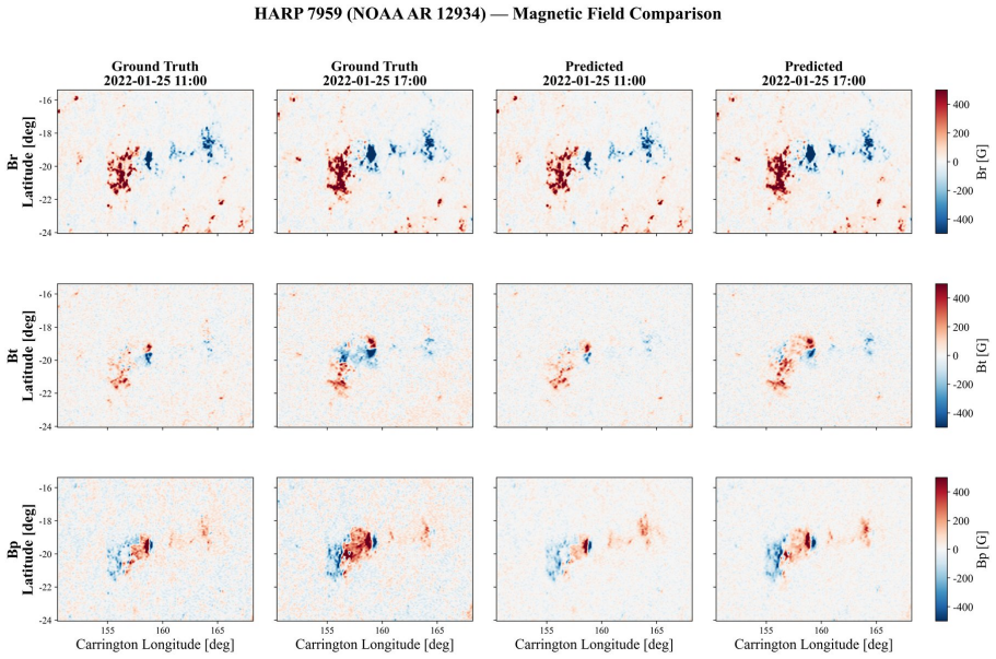
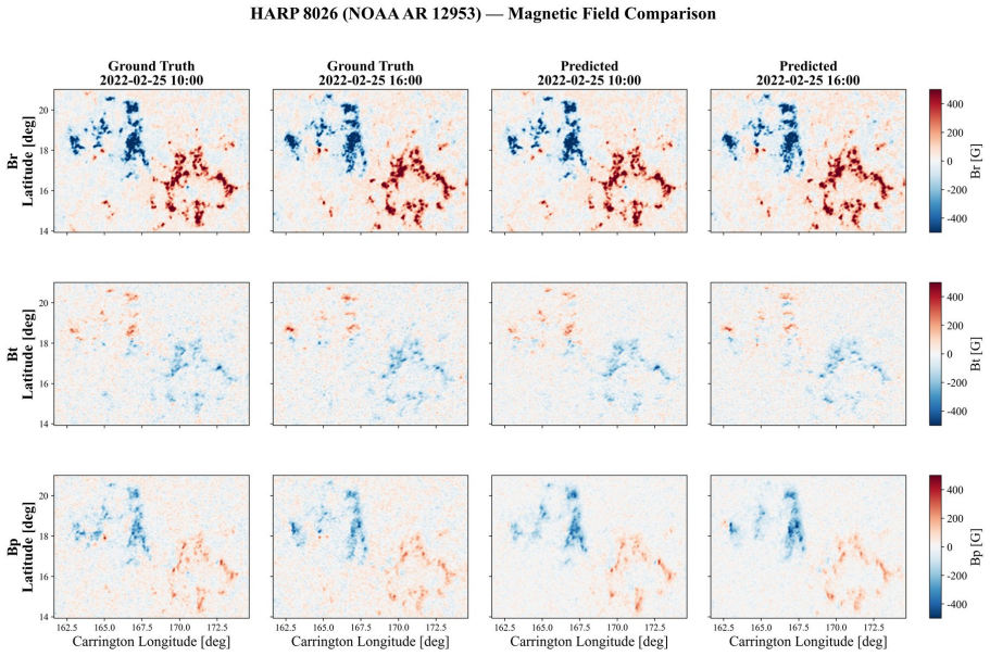
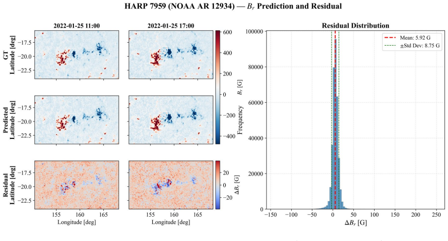
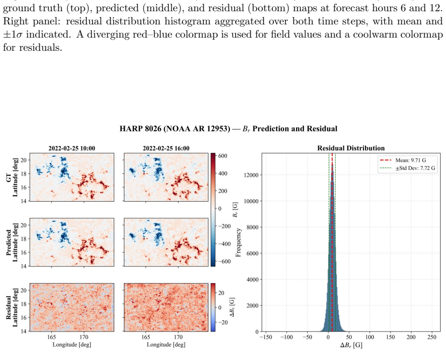
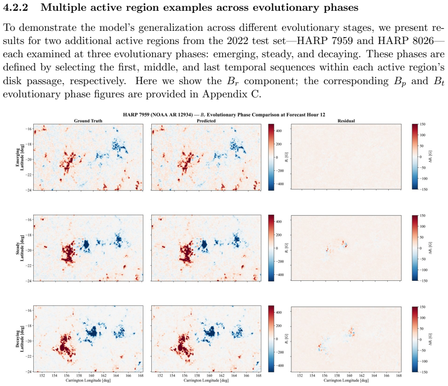
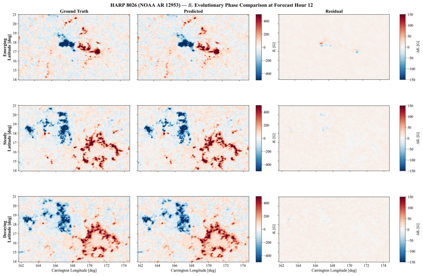
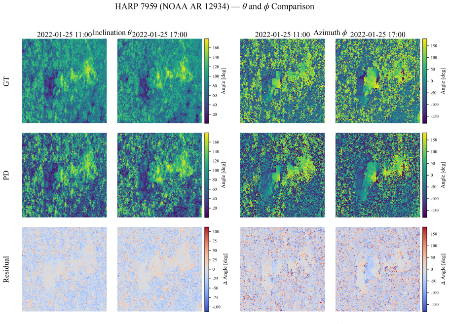
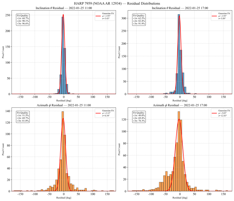
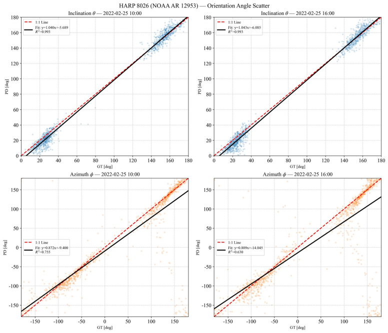
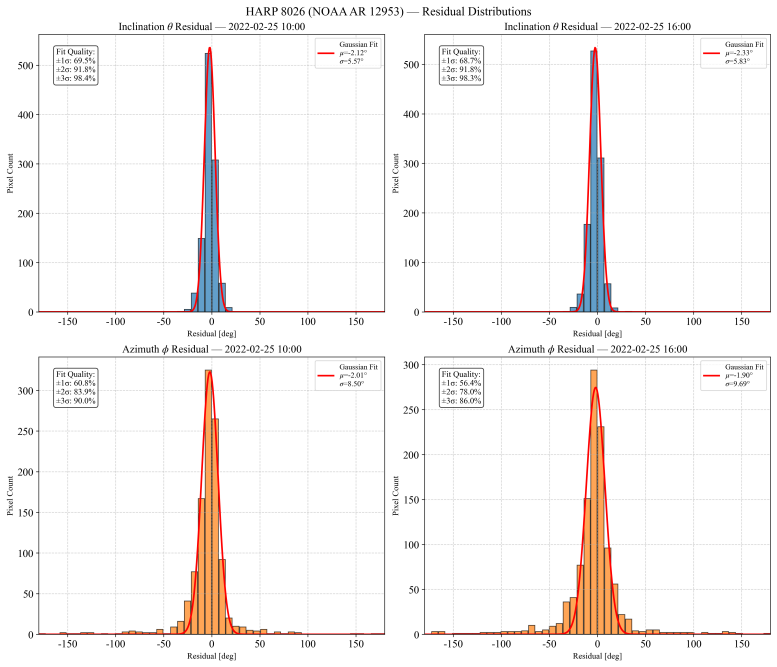
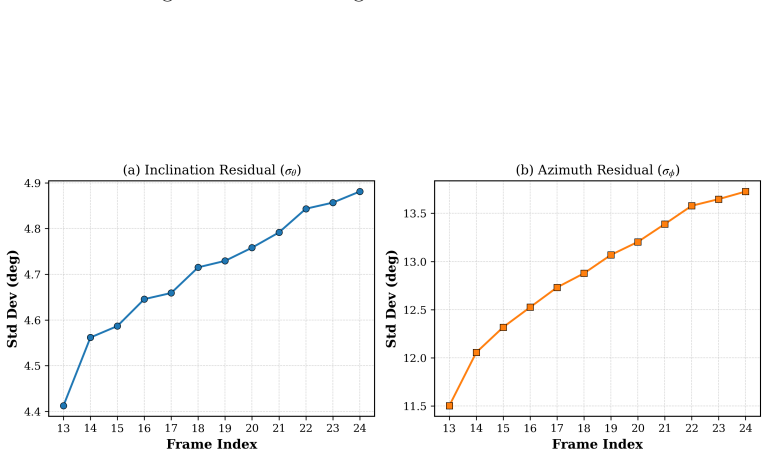
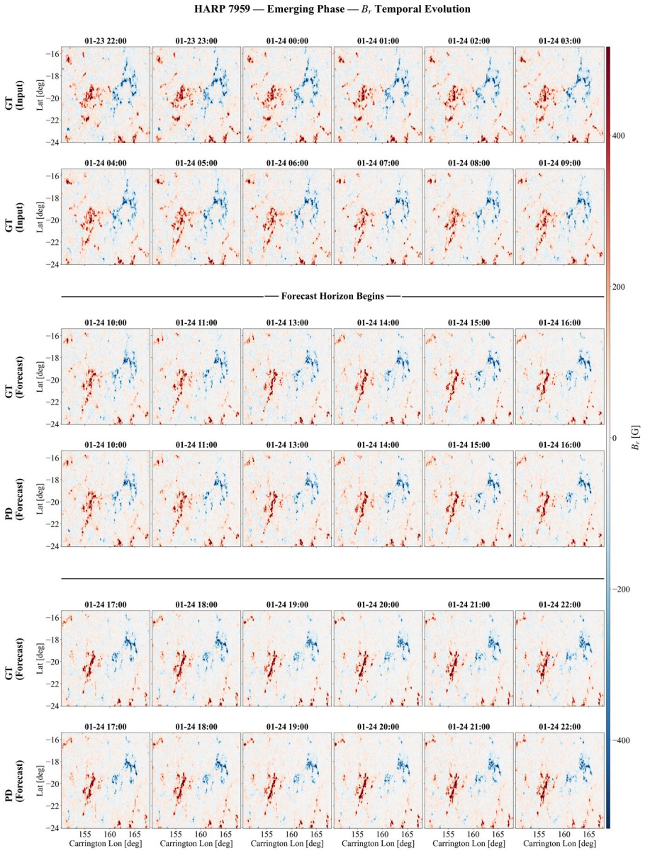
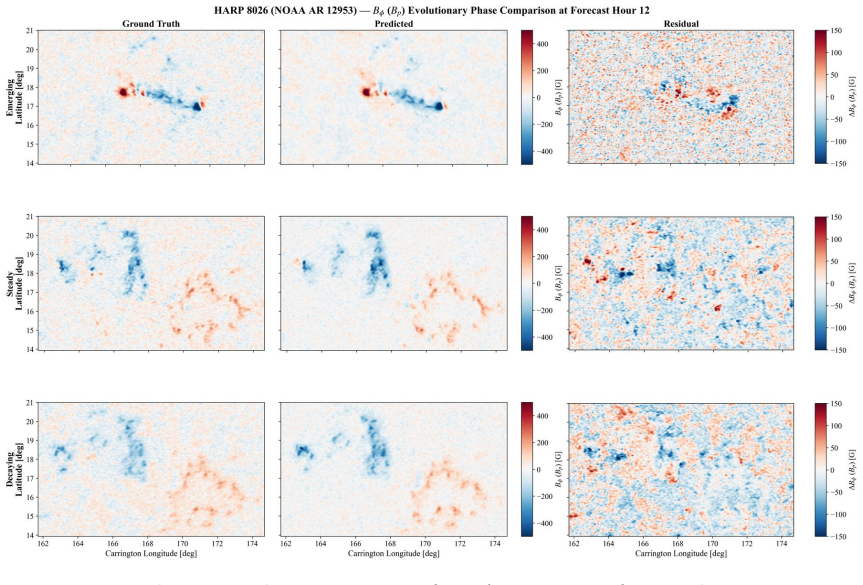
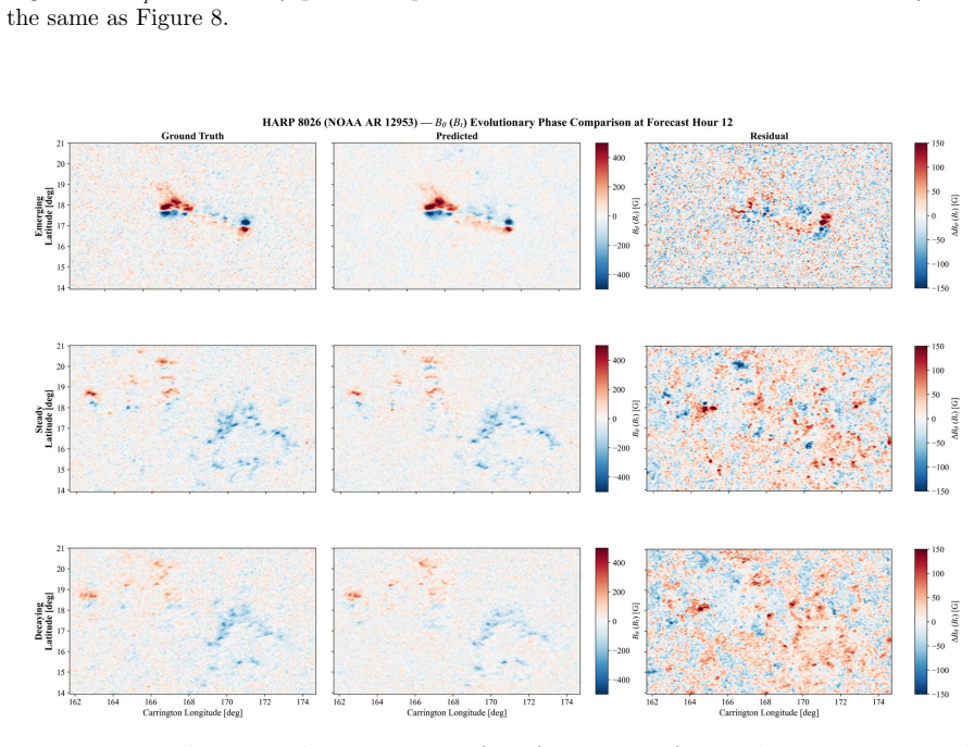
The proposed model, trained with dynamic masks of active regions and multi-parameter magnetic constraints, achieves horizon-averaged SSIM of 0.912 and CC of 0.998 for the radial magnetic field component Br, with RMSE between 13 and 21 G. Horizontal components reach SSIM values of 0.728 to 0.800 with CC above 0.895. Unsigned magnetic flux is predicted with an error of 7.82 percent (95 percent CI +/-0.11 percent). This demonstrates both strong performance in image space and consistency with magnetic diagnostics.
What carries the argument
Multi-parameter magnetic constraints added to the training loss, combined with dynamic masks on three-channel vector-magnetogram inputs, to enforce consistency across the 12-hour forecast horizon.
If this is right
- The radial component Br is forecasted with SSIM above 0.9 and correlation 0.998.
- Horizontal components maintain SSIM between 0.73 and 0.80 and correlation above 0.89.
- Unsigned flux errors remain at 7.82 percent with narrow confidence interval.
- The predictions stay consistent under the magnetic-parameter diagnostics used in the study.
- The method offers initial support for future space-weather forecasting pipelines.
Where Pith is reading between the lines
- The same constraint strategy could be tested on longer forecast horizons to check whether physical consistency holds beyond 12 hours.
- Adding further invariants such as force-free conditions might reduce residual inconsistencies in the horizontal components.
- Real-time integration with operational magnetogram streams would be a direct next step to assess practical utility.
- Comparison against unconstrained image-prediction baselines would quantify how much the magnetic terms improve flux preservation.
Load-bearing premise
That the added magnetic-parameter terms in the loss will keep the predicted vector fields consistent with observed physical quantities without creating new inconsistencies in the components.
What would settle it
An independent test set where the unsigned magnetic flux error exceeds 8 percent across a statistically significant number of active regions.
Figures


read the original abstract
Forecasting the dynamic evolution of solar magnetic fields is a critical technique for enabling space weather warnings. Addressing the limitations of existing methods in predicting all vector magnetic field components and in maintaining consistency with solar surface magnetic-field-related quantities, this study proposes a deep learning prediction method that integrates dynamic masks of active regions with multiple magnetic parameter constraints. By constructing a three-channel representation of vector magnetic fields, applying dynamic masks to enhance attention to strong-field regions, and incorporating multi-parameter magnetic parameter constraints, we developed an end-to-end short-term (12-hour) predictive model of solar vector magnetic field evolution. Using SDO/SHARP vector magnetogram data, the model predicts and analyses field evolution across all components. Quantitative evaluations demonstrate that our approach achieves horizon-averaged structural similarity index measure (SSIM) of 0.912 (per-hour range: 0.909--0.916) and correlation coefficient (CC) of 0.998 for the radial component Br (root-mean-square error (RMSE) 13.0--21.0 G); the horizontal components achieve Bphi SSIM 0.760--0.800 (CC 0.910--0.945, RMSE 38.5--50.0 G) and Btheta SSIM 0.728--0.750 (CC 0.895--0.920, RMSE 38.5--49.0 G). The model maintains unsigned magnetic flux prediction errors at 7.82% (95% confidence interval (CI): +/-0.11%). These results demonstrate strong image-domain performance together with consistency under the magnetic-parameter diagnostics used here, suggesting initial potential for supporting future space weather forecasting efforts.
Editorial analysis
A structured set of objections, weighed in public.
Referee Report
Summary. The manuscript proposes an end-to-end deep-learning model for 12-hour-ahead prediction of the three-component vector magnetic field in solar active regions. The approach combines a three-channel input representation of SDO/SHARP vector magnetograms, dynamic masks that focus attention on strong-field pixels, and multi-parameter magnetic constraints (including unsigned flux) added to the training loss. On held-out data the model is reported to achieve horizon-averaged SSIM = 0.912 and CC = 0.998 (RMSE 13–21 G) for Br, lower but still usable SSIM/CC values for the horizontal components, and a mean unsigned-flux error of 7.82 % (95 % CI ±0.11 %).
Significance. If the performance numbers and physical-consistency claims are reproducible, the work would supply a concrete, data-driven baseline for short-term vector-field evolution that could be tested against existing physics-based or empirical forecasting pipelines. The explicit inclusion of magnetic-parameter constraints in the loss is a methodological strength that distinguishes the study from purely image-domain regression approaches.
major comments (3)
- [§3, §4] §3 (Methods) and §4 (Results): the explicit mathematical form of the multi-parameter loss terms, their relative weights, and the mechanism by which the constraints are enforced at inference time are not stated. Without these equations it is impossible to verify that the reported flux-error reduction does not arise from compensating errors among the three vector components.
- [§4.2] §4.2 (Quantitative evaluation): the 95 % CI on the 7.82 % flux error is given, but the manuscript does not specify whether the interval accounts for the number of independent active regions, temporal autocorrelation within each region, or multiple random seeds. This directly affects the load-bearing claim that the constraints produce statistically reliable consistency.
- [§3.1] §3.1 (Network architecture): no description is supplied of the backbone network, the precise definition of the dynamic masks, or the training/validation/test split ratios. These omissions prevent independent assessment of whether the quoted SSIM/CC values are architecture-dependent or genuinely attributable to the magnetic constraints.
minor comments (2)
- [§4.1] The per-hour SSIM ranges are reported only for Br; analogous ranges should be supplied for Bθ and Bφ to allow direct comparison of component-wise temporal stability.
- [Figure captions] Figure captions should explicitly state the number of active regions and the exact forecast horizons used to compute the quoted aggregate metrics.
Simulated Author's Rebuttal
We thank the referee for the constructive and detailed comments, which highlight important aspects for improving reproducibility and statistical rigor. We address each major comment below and will revise the manuscript to incorporate clarifications and additional details where feasible.
read point-by-point responses
-
Referee: [§3, §4] §3 (Methods) and §4 (Results): the explicit mathematical form of the multi-parameter loss terms, their relative weights, and the mechanism by which the constraints are enforced at inference time are not stated. Without these equations it is impossible to verify that the reported flux-error reduction does not arise from compensating errors among the three vector components.
Authors: We agree that the explicit forms are necessary for verification. In the revised manuscript we will add the full mathematical definition of the composite loss (including the unsigned-flux term and any other magnetic-parameter penalties), the specific relative weights λ determined by cross-validation, and an explicit statement that the constraints operate exclusively during training. At inference the model performs unconstrained forward passes. We will also include a supplementary analysis of per-component residuals to demonstrate that the reported flux-error reduction is not produced by compensating errors across Br, Bθ and Bϕ. revision: yes
-
Referee: [§4.2] §4.2 (Quantitative evaluation): the 95 % CI on the 7.82 % flux error is given, but the manuscript does not specify whether the interval accounts for the number of independent active regions, temporal autocorrelation within each region, or multiple random seeds. This directly affects the load-bearing claim that the constraints produce statistically reliable consistency.
Authors: The reported 95 % CI was obtained via bootstrap resampling over the independent active regions in the held-out test set; five random seeds were used for training. We will add this description to §4.2. However, the original calculation did not explicitly block-bootstrap to account for temporal autocorrelation within each region. We will therefore revise the text to state the exact procedure used and to note this limitation; a full re-computation with clustered bootstrap would require additional experiments beyond the scope of a minor clarification and is left for future work. revision: partial
-
Referee: [§3.1] §3.1 (Network architecture): no description is supplied of the backbone network, the precise definition of the dynamic masks, or the training/validation/test split ratios. These omissions prevent independent assessment of whether the quoted SSIM/CC values are architecture-dependent or genuinely attributable to the magnetic constraints.
Authors: We will expand §3.1 with the requested details: the backbone is a U-Net architecture augmented with convolutional attention blocks; dynamic masks are binary maps generated by thresholding |Br| > 50 G (updated at each time step); and the data split is 70 % / 15 % / 15 % for training / validation / test, with active regions kept disjoint across splits to prevent leakage. These additions will allow readers to evaluate the contribution of the magnetic constraints independently of the architecture. revision: yes
Circularity Check
No circularity: standard DL training + independent test metrics
full rationale
The paper trains an end-to-end network on SDO/SHARP data with added loss terms for magnetic parameters and reports SSIM/CC/RMSE/flux error on held-out test magnetograms. No equation reduces a reported prediction to a fitted input by construction, no self-citation supplies a uniqueness theorem, and the evaluation metrics are external image and integral statistics computed after training. The derivation chain is therefore self-contained against external benchmarks.
Axiom & Free-Parameter Ledger
axioms (1)
- domain assumption A neural network trained on sequences of vector magnetograms can learn to predict future states when the loss includes both image similarity and magnetic-parameter terms.
Reference graph
Works this paper leans on
-
[1]
G. Aulanier, M. Janvier, and B. Schmieder. The standard flare model in three dimensions. i. strong-to-weak shear transition in post-flare loops. Astronomy and Astrophysics, 543: A110, 2012. doi: 10.1051/0004-6361/201219311
-
[2]
Predicting the evolution of photospheric magnetic field in solar active regions using deep learning
Liang Bai, Yi Bi, Bo Yang, Jun-Chao Hong, Zhe Xu, Zhen-Hong Shang, Hui Liu, Hai- Sheng Ji, and Kai-Fan Ji. Predicting the evolution of photospheric magnetic field in solar active regions using deep learning. Research in Astronomy and Astrophysics, 21(5):113,
-
[3]
doi: 10.1088/1674-4527/21/5/113
-
[4]
Scheduled sampling for sequence prediction with recurrent neural networks
Samy Bengio, Oriol Vinyals, Navdeep Jaitly, and Noam Shazeer. Scheduled sampling for sequence prediction with recurrent neural networks. In Advances in Neural Information Processing Systems, volume 28, pages 1171–1179, 2015
2015
-
[5]
M. G. Bobra and S. Couvidat. Solar flare prediction using sdo/hmi vector magnetic field data with a machine-learning algorithm. Astrophysical Journal, 798:135, 2015
2015
-
[6]
M. G. Bobra, X. Sun, J. T. Hoeksema, M. Turmon, Y. Liu, K. Hayashi, G. Barnes, and K. D. Leka. The Helioseismic and Magnetic Imager (HMI) Vector Magnetic Field Pipeline: SHARPs - Space-Weather HMI Active Region Patches.Sol. Phys., 289:3549–3578, Septem- ber 2014. doi: 10.1007/s11207-014-0529-3
-
[7]
Ruishuo Chen, Wutong Lu, Qi Hao, Yifan Meng, Pengfei Chen, and Chenxi Shi. Sta- tistical analyses of solar active region in SDO/HMI magnetograms detected by unsuper- vised machine learning method DSARD. arXiv preprint arXiv:2502.17990, feb 2025. doi: 10.48550/arXiv.2502.17990. URL https://arxiv.org/abs/2502.17990. 22 pages, 15 figures, submitted to ApJS
-
[8]
E. Covas, N. Peixinho, and J. Fernandes. Neural network forecast of the sunspot butterfly diagram. Solar Physics, 294(24):24, feb 2019. doi: 10.1007/s11207-019-1412-z. URL https://doi.org/10.1007/s11207-019-1412-z
-
[9]
Transfer learning in spatial–temporal forecasting of the solar magnetic field
Eurico Covas. Transfer learning in spatial–temporal forecasting of the solar magnetic field. Astronomische Nachrichten, 341(4), mar 2020. doi: 10.1002/asna.202013690. URL https://doi.org/10.1002/asna.202013690. First published: 30 March 2020
-
[10]
Y. Cui, R. Li, L. Zhang, Y. He, and H. Wang. Correlation between solar flare pro- ductivity and photospheric magnetic field properties. i. maximum horizontal gradient, length of neutral line, number of singular points. Solar Physics, 237(1):45–59, 2006. doi: 10.1007/s11207-006-0077-6
-
[11]
Y. Fan. MHD Equilibria and Triggers for Prominence Eruption, volume 415 of Astrophysics and Space Science Library, pages –. Springer, Cham, 2015. ISBN 978-3-319-10415-7. doi: 10.1007/978-3-319-10416-4\ 12. URL https://doi.org/10.1007/978-3-319-10416-4 12
-
[12]
G. H. Fisher, D. J. Bercik, B. T. Welsch, and H. S. Hudson. Global forces in eruptive solar flares: The lorentz force acting on the solar interior. Solar Physics, 277:59, 2012
2012
-
[13]
Hyun-Jin Jeong, Mingyu Jeon, Daeil Kim, Youngjae Kim, Ji-Hye Baek, Yong-Jae Moon, and Seonghwan Choi. Prediction of the next solar rotation synoptic maps using an artificial intelligence–based surface flux transport model. The Astrophysical Journal Supplement Series, 278(1):5, apr 2025. doi: 10.3847/1538-4365/adc447. 43
-
[14]
Prediction of time- evolving radial magnetic fields on the solar surface using deep learning
Hyun-Jin Jeong, Stefaan Poedts, Haopeng Wang, Ekatarina Dineva, Panagiotis Gonidakis, Francesco Carella, George Miloshevich, Luis Linan, and Harim Lee. Prediction of time- evolving radial magnetic fields on the solar surface using deep learning. The Astrophysical Journal Letters, 989(2):L31, aug 2025. doi: 10.3847/2041-8213/adf5c7
-
[15]
Jiang, R
J. Jiang, R. H. Cameron, and M. Sch¨ ussler. Effects of the scatter in sunspot group tilt angles on the large-scale magnetic field at the solar surface. Astrophysical Journal, 791(1): 5, 2014
2014
-
[16]
J. Jiang, D. H. Hathaway, R. H. Cameron, S. K. Solanki, L. Gizon, and L. Upton. Magnetic flux transport at the solar surface. Space Science Reviews, 186(1-4):491–523, dec 2014. doi: 10.1007/s11214-014-0083-1. URL https://doi.org/10.1007/s11214-014-0083-1
-
[17]
E. K. J. Kilpua, N. Lugaz, M. L. Mays, and M. Temmer. Forecasting the structure and orientation of earthbound coronal mass ejections. Space Weather, 17(4):498–526, 2019. doi: 10.1029/2018SW001944
-
[18]
Adam: A method for stochastic optimization
Diederik P Kingma and Jimmy Ba. Adam: A method for stochastic optimization. arXiv preprint arXiv:1412.6980, 2014
Pith/arXiv arXiv 2014
-
[19]
K. D. Leka and G. Barnes. Photospheric magnetic field properties of flaring versus flare- quiet active regions. ii. discriminant analysis. Astrophysical Journal, 595:1296, 2003
2003
-
[20]
Francesco Pio Ramunno, Hyun-Jin Jeong, Stefan Hackstein, Andr´ e Csillaghy, Svyatoslav Voloshynovskiy, and Manolis K. Georgoulis. Magnetogram-to-magnetogram: Generative forecasting of solar evolution. arXiv preprint arXiv:2407.11659, jul 2024. doi: 10.48550/ arXiv.2407.11659. URL https://arxiv.org/abs/2407.11659. Conference paper accepted for oral present...
arXiv 2024
-
[21]
Y. Su, A. Veronig, G. Holman, et al. Imaging coronal magnetic-field reconnection in a solar flare. Nature Physics, 9:489–493, 2013. doi: 10.1038/nphys2675
-
[22]
Flare-productive active regions
Shin Toriumi and Haimin Wang. Flare-productive active regions. Living Reviews in Solar Physics, 16(1):3, 2019. doi: 10.1007/s41116-019-0019-7. URL https://link.springer.com/ article/10.1007/s41116-019-0019-7
-
[23]
ADS Bibcode: 2013ApJ...773...93S The Astropy Collaboration, Price-Whelan, A
L. Upton and D. H. Hathaway. Predicting the sun’s polar magnetic fields with a surface flux transport model. The Astrophysical Journal, 780(1):5, 2014. doi: 10.1088/0004-637X/ 780/1/5
-
[24]
H. Wu, Z. Yao, J. Wang, and M. Long. Motionrnn: A flexible model for video prediction with spacetime-varying motions. 2021
2021
-
[25]
G. Yang, Y. Xu, W. D. Cao, et al. Photospheric shear flows along the magnetic neutral line of active region 10486 prior to an x10 flare. Astrophysical Journal, 617:L151, 2004. 44
2004
discussion (0)
Sign in with ORCID, Apple, or X to comment. Anyone can read and Pith papers without signing in.