Data-driven methods for computation of optimal linear response in high-dimensional dynamical systems
Pith reviewed 2026-06-27 23:01 UTC · model grok-4.3
The pith
Kernel-smoothed approximations of transfer operators enable data-driven optimization of infinitesimal perturbations to manipulate system spectra.
A machine-rendered reading of the paper's core claim, the machinery that carries it, and where it could break.
Core claim
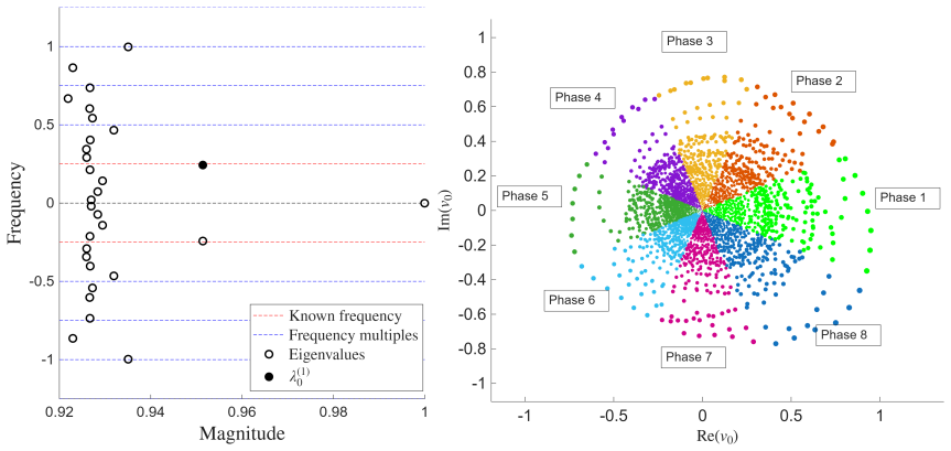
Kernel-smoothed approximations of the transfer and Koopman operators, built from trajectory data, are inserted into a spectral optimization problem whose solution is the optimal infinitesimal perturbation that realizes any prescribed manipulation of the spectrum, including increases in frequency or reductions in decay rate for eigenvalues tied to almost-cycles or almost-invariant sets.
What carries the argument
Kernel-smoothed approximations of the transfer and Koopman operators that turn spectral manipulation into a tractable optimization problem solved from data.
If this is right
- The optimization can be solved to increase frequency or suppress decay of correlations for almost-cycles identified by the approximated operator.
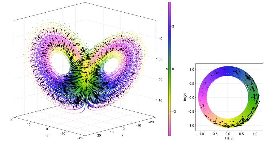
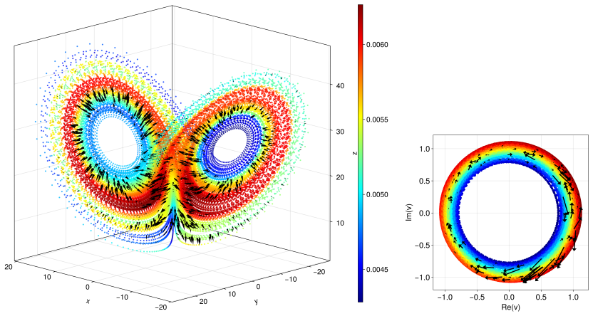
- Optimal-response vector fields constructed from the same data visualize the physical effect of the perturbation under any chosen observations.
- The procedure scales to high-dimensional trajectory data, as shown by its application to an Earth system model for El Nino Southern Oscillation.
- The resulting perturbations are nontrivial yet consistent with the target dynamical objectives in the tested periodic, chaotic, and climate examples.
Where Pith is reading between the lines
- If the transfer from approximation to true system holds, the same workflow could locate targeted adjustments that lengthen or shorten specific climate oscillations.
- The vector-field construction might be reused to interpret how a chosen perturbation affects statistics under observations different from those used to build the operator.
- Repeating the procedure on systems whose exact linear response is known analytically would directly test how much approximation error is tolerable before the computed perturbation loses its optimality.
Load-bearing premise
The kernel-smoothed operator approximations remain accurate enough that perturbations optimal for the approximation remain optimal for the true nonlinear system.
What would settle it
Take the perturbation found from the approximated operators, apply it to the original dynamical system, and measure whether the relevant eigenvalues of the true transfer operator move exactly as the optimization predicted.
Figures


read the original abstract
We develop a data-driven framework for estimating optimal linear response of nonlinear dynamical systems. Our approach is based on kernel-smoothed approximations of the transfer/Koopman operators of the system, built from possibly high-dimensional observations along trajectories. Combining these operator approximations with the theory developed in [Antown et al. (2018), J. Stat. Phys., 170(6), 1051-1087], we formulate a computationally tractable optimization problem for the optimal infinitesimal perturbation realising any desired manipulation of the spectrum. We also introduce a notion of optimal-response vector fields for visualising, and physically interpreting, the system's response to the optimal perturbation under arbitrary observations. Our focus is on finding perturbations that optimally increase the frequency or optimally suppress the decay of correlations of almost-cycles or almost-invariant sets associated with the eigenvalues of the kernel-smoothed transfer operator. We illustrate our approach with applications to low-dimensional periodic and chaotic systems, as well as a high-dimensional example involving the El Nino Southern Oscillation in a comprehensive Earth system model. In these examples our approach discovers nontrivial optimal perturbations of the system, which are post hoc natural and consistent with the desired dynamical objectives.
Editorial analysis
A structured set of objections, weighed in public.
Referee Report
Summary. The paper develops a data-driven framework for estimating optimal linear response in nonlinear dynamical systems. It uses kernel-smoothed approximations of transfer/Koopman operators constructed from trajectory data (possibly high-dimensional), combines these with the optimization theory of Antown et al. (2018) to pose a tractable problem for infinitesimal perturbations that achieve desired spectral manipulations (e.g., increasing frequency or suppressing correlation decay of almost-cycles), and introduces optimal-response vector fields for interpretation. The method is illustrated on low-dimensional periodic/chaotic systems and a high-dimensional ENSO example in an Earth system model, where the discovered perturbations are reported as nontrivial yet physically natural.
Significance. If the kernel approximations are shown to yield perturbations whose spectral effects transfer to the true nonlinear operator, the framework would offer a practical, observation-based route to optimal control of spectral properties in high-dimensional systems, with direct relevance to climate dynamics and chaos control. The combination of data-driven operator learning with an external optimization theory is a natural extension, and the introduction of optimal-response vector fields provides a useful interpretive tool.
major comments (3)
- [Formulation of the optimization problem] Formulation of the optimization problem (section referenced in the abstract): the kernel-smoothed operator is used to define the optimization problem, but no a-priori error bound or Lipschitz-type control is given on how the approximation error affects the non-convex optimizer; consequently it is not shown that a perturbation optimal for the smoothed operator remains near-optimal (or even produces the desired spectral shift) when the true transfer operator is substituted.
- [Numerical examples] Numerical examples section: the ENSO and low-dimensional examples report that the discovered perturbations are 'post hoc natural,' yet no quantitative metric (e.g., table of eigenvalue displacements or correlation-decay rates) compares the effect of the optimal vector field under the kernel-smoothed operator versus the true underlying dynamics or a finer-resolution reference operator.
- [Optimal-response vector fields] Definition of optimal-response vector fields: the construction appears to rely on the same kernel-smoothed operator used for the optimization; without an accompanying error analysis or sensitivity test, it is unclear whether these vector fields correctly represent the response of the original nonlinear system under arbitrary observations.
minor comments (2)
- Notation for the kernel bandwidth/smoothing parameter is introduced without an explicit symbol in the abstract and early sections; a consistent symbol and discussion of its selection would improve readability.
- The manuscript cites Antown et al. (2018) for the core optimization theory; a brief self-contained recap of the relevant theorem (or at least the precise statement used) would help readers who have not consulted the reference.
Simulated Author's Rebuttal
We thank the referee for the thorough and constructive report. We address each major comment below and outline the revisions we will make.
read point-by-point responses
-
Referee: [Formulation of the optimization problem] the kernel-smoothed operator is used to define the optimization problem, but no a-priori error bound or Lipschitz-type control is given on how the approximation error affects the non-convex optimizer; consequently it is not shown that a perturbation optimal for the smoothed operator remains near-optimal (or even produces the desired spectral shift) when the true transfer operator is substituted.
Authors: We agree that rigorous a-priori bounds on the propagation of kernel approximation error through the non-convex spectral optimization would be desirable. Deriving such bounds appears technically difficult because the problem is non-convex and the underlying operators are infinite-dimensional. In the revised manuscript we will add a dedicated discussion of this limitation together with numerical sensitivity experiments that vary kernel bandwidth, sample size, and regularization; these tests will quantify how much the computed optimal perturbations and resulting eigenvalue shifts change under controlled perturbations of the approximated operator. revision: partial
-
Referee: [Numerical examples] the ENSO and low-dimensional examples report that the discovered perturbations are 'post hoc natural,' yet no quantitative metric (e.g., table of eigenvalue displacements or correlation-decay rates) compares the effect of the optimal vector field under the kernel-smoothed operator versus the true underlying dynamics or a finer-resolution reference operator.
Authors: The observation is correct. For the low-dimensional periodic and chaotic examples we will insert tables that directly compare the eigenvalue displacements and correlation-decay rates obtained from the kernel-smoothed operator against the exact transfer operator (or a high-resolution reference). For the high-dimensional ENSO example, an exact operator is unavailable; we will instead report results obtained from several independent long trajectories and from cross-validation across different kernel parameters to demonstrate consistency of the discovered perturbations. revision: yes
-
Referee: [Optimal-response vector fields] the construction appears to rely on the same kernel-smoothed operator used for the optimization; without an accompanying error analysis or sensitivity test, it is unclear whether these vector fields correctly represent the response of the original nonlinear system under arbitrary observations.
Authors: We will revise the section on optimal-response vector fields to include explicit sensitivity tests with respect to kernel bandwidth and data subsampling. We will also add a clarifying paragraph stating that the vector fields are constructed from the data-driven approximation and therefore inherit its limitations; the tests will illustrate the degree of stability of the visualized fields under these variations. revision: yes
Circularity Check
No circularity; derivation combines external theory with data-driven approximations
full rationale
The paper constructs kernel-smoothed transfer/Koopman operator approximations from trajectory data and invokes the optimization framework of the external Antown et al. (2018) reference to set up a tractable problem for optimal perturbations. No step reduces a claimed result to a fitted quantity or self-defined input by construction, no load-bearing self-citation chain exists, and the derivation remains self-contained against the stated external benchmark and data-driven inputs. The transfer of optimality from the smoothed operator to the true system is an assumption separate from any definitional circularity.
Axiom & Free-Parameter Ledger
free parameters (1)
- kernel bandwidth / smoothing parameter
axioms (1)
- domain assumption The theory developed in Antown et al. (2018) applies directly to the kernel-smoothed operator approximations.
invented entities (1)
-
optimal-response vector fields
no independent evidence
Reference graph
Works this paper leans on
-
[1]
M. Ghil and V. Lucarini. The physics of climate variability and climate change. Rev. Mod. Phys., 92:035002, 2020. doi:10.1103/RevModPhys.92.035002
-
[2]
V. Lucarini, F. Ragone, and F. Lunkeit. Predicting climate change using re- sponse theory: Global averages and spatial patterns.J. Stat. Phys., 166:1036– 1064, 2017. doi:10.1007/s10955-016-1506-z
-
[3]
D. Ruelle. Differentiation of SRB states.Commun. Math. Phys., 187:227–241,
-
[4]
doi:10.1007/s002200050134
-
[6]
V. Baladi. Linear response, or else, 2014. URLhttps://arxiv.org/abs/1408
2014
-
[7]
H. B. Callen and T. A. Welton. Irreversibility and generalized noise.Phys. Rev., 83(1):34–40, 1951. doi:10.1103/PhysRev.83.34
-
[8]
R. Kubo. The fluctuation–dissipation theorem.Rep. Prog. Phys., 29:255–284,
-
[9]
doi:10.1088/0034-4885/29/1/306
-
[10]
R. H. Kraichnan. Classical fluctuation–relaxation theorem.Phys. Rev., 113(5),
-
[11]
doi:10.1103/PhysRev.113.1181. 30
-
[13]
G. Gallavotti and E. G. D. Cohen. Dynamic ensembles in stationary states. Phys. Rev. Lett., 74(14):2694–2697, 1995. doi:10.1103/PhysRevLett.74.2694
-
[14]
G. Gallavotti. Onsager hypothesis: Onsager reciprocity and fluctuation–dissipation theorem.J. Stat. Phys., 84(5/6):899–925, 1996. doi:10.1007/bf02174123
-
[15]
L.-S. Young. What are SRB measures, and which dynamical systems have them?J. Stat. Phys., 108:733–754, 2002. doi:10.1023/a:1019762724717
-
[16]
R. Bowen and D. Ruelle. The ergodic theory of Axiom A flows.Inventiones Mathematicae, 29:181–202, 1975. doi:10.1007/bf01389848
-
[17]
S. Gou¨ ezel and C. Liverani. Banach spaces adapted to Anosov systems.Ergod. Theory Dyn. Syst., 26:189–217, 2006. doi:10.1017/s0143385705000374
-
[18]
R. V. Abramov and A. Majda. New approximations and tests of linear fluctuation-response for chaotic nonlinear forced-dissipative dynamical systems. J. Nonlinear Sci., 18:303–341, 2008. doi:10.1007/s00332-007-9011-9
-
[19]
Baladi and D
V. Baladi and D. Smania. Smooth deformations of piecewise expanding uni- modal maps.Discrete and Continuous Dynamical Systems, 23(3):685–703,
-
[20]
doi:10.3934/dcds.2009.23.685
-
[21]
M. Hairer and A. J. Majda. A simple framework to justify linear response theory.Nonlinearity, 23(4):909–922, 2010. doi:10.1088/0951-7715/23/4/008
-
[22]
V. Baladi, T. Kuna, and V. Lucarini. Linear and fractional response for the srb measure of smooth hyperbolic attractors and discontinuous observables. Nonlinearity, 30(3), 2017. doi:10.1088/1361-6544/aa5b13
-
[23]
V. Baladi and M. Todd. Linear response for intermittent maps.Communica- tions in Mathematical Physics, 347, 2016. doi:10.1007/s00220-016-2577-z
-
[24]
C.L. Wormell and G.A. Gottwald. On the validity of linear response theory in high-dimensional deterministic dynamical systems.Journal of Statistical Physics, 172, 2018. doi:10.1007/s10955-018-2106-x
-
[25]
G. A. Gottwald, C. Wormell, and J Wouters. On spurious detection of linear response and misuse of the fluctuation-dissipation theorem in fi- nite time series.Physica D Nonlinear Phenomena, 331:89–101, 2016. doi:10.1016/j.physd.2016.05.010
-
[26]
A rigor- ous computational approach to linear response.Nonlinearity, 31(3):1073–1109, 2018
Wael Bahsoun, Stefano Galatolo, Isaia Nisoli, and Xiaolong Niu. A rigor- ous computational approach to linear response.Nonlinearity, 31(3):1073–1109, 2018. 31
2018
-
[27]
N. Chandramoorthy and Q. Wang. Efficient computation of linear response of chaotic attractors with one-dimensional unstable manifolds.SIAM J. Appl. Dyn. Syst., 21(2):735–781, 2022. doi:10.1137/21m1405599
-
[28]
A. Ni. Fast differentiation of hyperbolic chaos.Archive for Rational Mechanics and Analysis, 250(1), 2026
2026
-
[29]
G. Froyland and M. Phalempin. Optimal linear response for Anosov diffeomor- phisms, 2025. URLhttps://arxiv.org/abs/2504.16532
Pith/arXiv arXiv 2025
-
[30]
T. Bell. Climate sensitivity from fluctuation dissipation: Some simple model tests.J. Atmos. Sci, 37(8):1700–1708, 1980. doi:10.1175/1520- 0469(1980)037<1700:csffds>2.0.co;2
-
[31]
A. S. Gritsoun. Fluctuation-dissipation theorem on attractors of atmo- spheric models.Russ. J. Numer. Anal. Math. Modelling, 16(2):115–133, 2001. doi:10.1515/rnam-2001-0203
-
[32]
A. S. Gritsoun, G. Branstator, and V. P. Dymnikov. Construction of the lin- ear response operator of an atmospheric general circulation model to small external forcing.Russ. J. Numer. Anal. Math. Modelling, 17(5):399–416, 2002. doi:10.1515/rnam-2002-0503
-
[33]
A. J. Majda, R. V. Abramov, and M. J. Grote.Information Theory and Stochas- tics for Multiscale Nonlinear Systems, volume 25 ofCRM Monograph Series. Americal Mathematical Society, Providence, 2005
2005
-
[34]
A. J. Majda, R. Abramov, and B. Gershgorin. High skill in low-frequency cli- mate response through fluctuation dissipation theorems despite structural insta- bility.Proc. Natl. Acad. Sci, 107(2):581–586, 2010. doi:10.1073/pnas.091299710
-
[35]
M. Dellnitz and O. Junge. On the approximation of complicated dynamical be- havior.SIAM J. Numer. Anal., 36:491, 1999. doi:10.1137/s0036142996313002
-
[36]
Sch¨ utte, W
Ch. Sch¨ utte, W. Huisinga, and P. Deuflhard. Transfer operator approach to conformational dynamics in biomolecular systems. In B. Fiedler, editor,Ergodic Theory, Analysis, and Efficient Simulation of Dynamical Systems, pages 191–
-
[37]
doi:10.1007/978-3-642-56589-2 9
Springer-Verlag, Berlin, 2001. doi:10.1007/978-3-642-56589-2 9
-
[38]
I. Mezi´ c. Spectral properties of dynamical systems, model reduction and decom- positions.Nonlinear Dyn., 41:309–325, 2005. doi:10.1007/s11071-005-2824-x
-
[39]
I. Mezi´ c and A. Banaszuk. Comparison of systems with complex behavior. Phys. D., 197:101–133, 2004. doi:10.1016/j.physd.2004.06.015
-
[40]
S. E. Otto and C. W. Rowley. Koopman operators for estimation and control of dynamical systems.Annu. Rev. Control Robot. Auton. Syst., 4:59–87, 2021. doi:10.1146/annurev-control-071020-010108. 32
-
[41]
M. Colbrook. The multiverse of dynamic mode decomposition algorithms. InHandbook of Numerical Analysis, pages 127–230. Amsterdam, 2024. doi:10.1016/bs.hna.2024.05.004
-
[42]
S. L. Brunton, M. Budisi´ c, E. Kaiser, and J. N. Kutz. Modern Koop- man theory for dynamical systems.SIAM Rev., 64(2):229–340, 2022. doi:10.1137/21m1401243
-
[43]
V. Baladi.Dynamical Zeta Functions and Dynamical Determi- nants for Hyperbolic Maps: A Functional Approach. Springer, 2018. doi:https://doi.org/10.1007/978-3-319-77661-3
-
[44]
Santos Guti´ errez and V
M. Santos Guti´ errez and V. Lucarini. On some aspects of the response to stochastic and deterministic forcings.J. Phys. A: Math. Theor., art. 425002,
-
[45]
doi:10.1088/1751-8121/ac90fd
-
[46]
N. Zagli, M. J. Colbrook, V. Lucarini, I. Mezi’c, and J. Moroney. Bridging the gap between Koopmanism and response theory: Using natural variability to predict forced response.SIAM J. Appl. Dyn. Syst., 25(1):196–229, 2026. doi:10.1137/24m1699206
-
[47]
V. Lucarini, M. Santos Guti´ errez, J. Moroney, and N. Zagli. A general frame- work for linking free and forced fluctuations via Koopmanism.Chaos Solitons Fractals, 202(Part 1):117540, 2026. doi:10.1016/j.chaos.2025.117540
-
[48]
M. O. Williams, I. G. Kevrekidis, and C. W. Rowley. A data-driven approxi- mation of the Koopman operator: Extending dynamic mode decomposition.J. Nonlinear Sci., 25(6):1307–1346, 2015. doi:10.1007/s00332-015-9258-5
-
[50]
G. Froyland, C. Gonz´ alez-Tokman, and A. Quas. Detecting isolated spectrum of transfer and Koopman operators with Fourier analytic tools.J. Comput. Dyn., 1(2):249–278, 2014. doi:10.3934/jcd.2014.1.249
-
[51]
M. Porte. Linear response for Dirac observables of Anosov diffeomor- phisms.Discrete and Continuous Dynamical Systems, 39(4):1799–1819, 2019. doi:10.3934/dcds.2019078
-
[52]
Froyland
G. Froyland. Statistically optimal almost-invariant sets.Phys. D., 200:205–219,
-
[53]
doi:10.1016/j.physd.2004.11.008
-
[54]
G. Froyland, D. Giannakis, B. Lintner, M. Pike, and J. Slawinska. Spectral analysis of climate dynamics with operator-theoretic approaches.Nat. Com- mun., 12:6570, 2021. doi:10.1038/s41467-021-26357-x
-
[55]
M. M. Castro and G. Froyland. On the structure of complex spectra and eigenfunctions of transfer and Koopman operators, 2025. URLhttps://arxiv. org/abs/2505.05770. 33
Pith/arXiv arXiv 2025
-
[56]
Froyland and N
G. Froyland and N. Santitissadeekorn. Optimal mixing enhancement.SIAM Journal on Applied Mathematics, pages 1444–1470, 2017
2017
-
[57]
Froyland, P
G. Froyland, P. Koltai, and M. Stahn. Computation and optimal perturbation of finite-time coherent sets for aperiodic flows without trajectory integration. SIAM Journal on Applied Dynamical Systems, 19(3):1659–1700, 2020
2020
-
[58]
F. Antown, D. Dragiˇ cevi´ c, and G. Froyland. Optimal linear responses for Markov chains and stochastically perturbed dynamical systems.J. Stat. Phys., 170(6):1051–1087, 2018. doi:10.1007/s10955-018-1985-1
-
[59]
F. Antown, G. Froyland, and S. Galatolo. Optimal linear response for Markov Hilbert–Schmidt integral operators and stochastic dynamical systems.J. Non- linear Sci., 32:79, 2022. doi:10.1007/s00332-022-09839-0
-
[60]
M. Santos Guti´ erez, N. Zagli, and G. Carigi. Markov matrix perturbations to optimize dynamical and entropy functionals, 2025. URLhttps://arxiv.org/ abs/2507.14040
arXiv 2025
-
[61]
S. Das and D. Giannakis. Delay-coordinate maps and the spectra of Koopman operators.J. Stat. Phys., 175(6):1107–1145, 2019. doi:10.1007/s10955-019- 02272-w
-
[62]
D. Giannakis. Delay-coordinate maps, coherence, and approximate spectra of evolution operators.Res. Math. Sci., 8:8, 2021. doi:10.1007/s40687-020-00239- y
-
[63]
F. Takens. Detecting strange attractors in turbulence. InDynamical Systems and Turbulence, volume 898 ofLecture Notes in Mathematics, pages 366–381. Springer, Berlin, 1981. doi:10.1007/bfb0091924
-
[65]
P. J. Webster, A. Moore, J. Loschnigg, and M. Leban. Coupled ocean dy- namics in the Indian Ocean during 1997–98.Nature, 401:356–360, 1999. doi:10.1038/43848
-
[66]
T. Sauer, J. A. Yorke, and M. Casdagli. Embedology.J. Stat. Phys., 65(3–4): 579–616, 1991. doi:10.1007/bf01053745
-
[67]
J. C. Robinson. A topological delay embedding theorem for infinite-dimensional dynamical systems.Nonlinearity, 18(5):2135–2143, 2005. doi:10.1088/0951- 7715/18/5/013
-
[68]
J. C. Robinson. A topological time-delay embedding theorem for infinite- dimensional cocycle dynamical systems.Discrete Cont. Dyn. Syst. Ser. B, 9 (3&4):731–741, 2008. doi:10.3934/dcdsb.2008.9.731. 34
-
[69]
E. R. Deyle and G. Sugihara. Generalized theorems for nonlinear state space re- construction.PLoS ONE, 6(3):e18295, 2011. doi:10.1371/journal.pone.0018295
-
[70]
E. A. Nadaraya. On estimating regression.Theory Probab. Appl., 9(1):141–142,
-
[71]
G. S. Watson. Smooth regression analysis.Sankhya Ser. A, 26(4):359–372, 1964
1964
-
[72]
E. M. Stein.Harmonic Analysis: Real-Variable Methods, Orthogonality, and Oscillatory Integrals, volume 43 ofPrinceton Mathematical Series. Princeton University Press, Princeton, 1993
1993
-
[73]
Haj lasz, P
P. Haj lasz, P. Koskela, and H. Tuominen. Sobolev embeddings, extensions and measure density condition.Journal of Functional Analysis, 254(5):1217–1234,
-
[74]
ISSN 0022-1236. doi:10.1016/j.jfa.2007.11.020
-
[75]
Giannakis and M
D. Giannakis and M. J. Latifi-Jebelli. Kernel smoothing operators on thick open domains.Anal. Math., 2026. In press
2026
-
[76]
J. Bj¨ orn, P. MacManus, and N. Shanmugalingam. Fat sets and pointwise bound- ary estimates forp-harmonic functions in metric spaces.J. Anal. Math., 85: 339–369, 2001. doi:10.1007/bf02788087
-
[77]
J. Canto, L. Ihnatsyeva, J. Lehrb¨ ack, and A. V. V¨ ah¨ akangas. Capaci- ties and density conditions in metric spaces.Potential Anal., 62(2), 2025. doi:10.1007/s11118-024-10137-5
-
[78]
R. Z. Khas’minskii. The behavior of a self-oscillating system acted upon by slight noise.Journal of Applied Mathematics and Mechanics, 27(4):1035–1044,
-
[79]
doi:https://doi.org/10.1016/0021-8928(63)90184-9
ISSN 0021-8928. doi:https://doi.org/10.1016/0021-8928(63)90184-9
-
[80]
Y. I. Kifer. On small random perturbations of some smooth dynamical systems.Math. USSR-Izv., 8:1083–1107, 1974. doi:10.1070/IM1974v008n05ABEH002139
-
[81]
S. M. Ulam.Problems in Modern Mathematics. Dover Publications, Mineola, 1964
1964
-
[82]
J. G. Kemeny and J. L. Snell.Finite Markov Chains. Springer New York, 1983
1983
-
[83]
G. Froyland, C. P. Rock, and K. Sakellariou. Sparse eigenbasis approximation: Multiple feature extraction across spatiotemporal scales with application to co- herent set identification.Communications in Nonlinear Science and Numerical Simulation, 77:81–107, 2019. doi:https://doi.org/10.1016/j.cnsns.2019.04.012
-
[84]
G. Froyland, D. Giannakis, E. Luna, and J. Slawinska. Revealing trends and persistent cycles of non-autonomous systems with operator-theoretic tech- niques: Applications to past and present climate dynamics.Nat. Commun., 15: 4268, 2024. doi:10.1038/s41467-024-48033-6. 35
discussion (0)
Sign in with ORCID, Apple, or X to comment. Anyone can read and Pith papers without signing in.