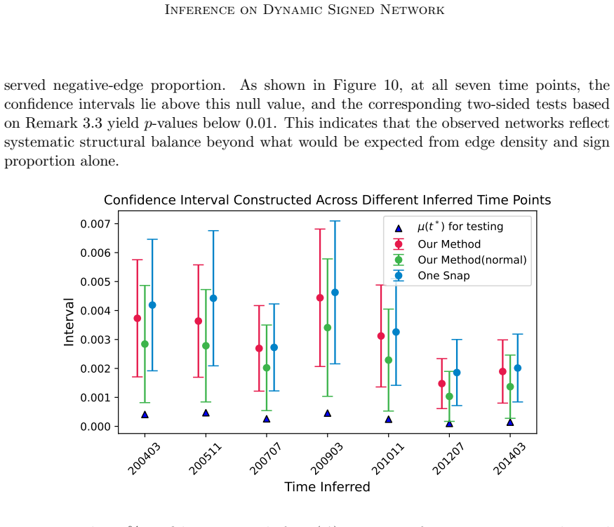
Inference for Balance in Dynamic Signed Networks
Pith reviewed 2026-06-27 17:43 UTC · model grok-4.3
The pith
Kernel smoothing enables inference on structural balance at any time in dynamic signed networks.
A machine-rendered reading of the paper's core claim, the machinery that carries it, and where it could break.
Core claim
In the dynamic signed graphon model, the kernel-smoothed estimator of the structural balance measure at a target time admits a studentized inference procedure whose finite-sample distribution is approximated to higher order by an Edgeworth expansion; temporal smoothing reduces the variance contribution from observation noise up to smoothing bias and time-discretization error.
What carries the argument
The kernel-smoothed estimator of the structural balance measure under the dynamic signed graphon model, which aggregates signed edges across a local time window.
If this is right
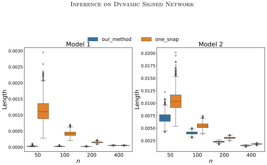
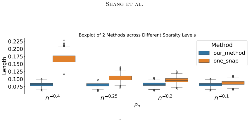
- Temporal smoothing reduces variance of the balance estimator in sparse networks.
- The procedure yields valid inference at target times that do not coincide with any observed snapshot.
- The Edgeworth expansion supplies a higher-order correction to the normal approximation for the studentized statistic.
- The method applies directly to observed dynamic networks such as international relations data.
Where Pith is reading between the lines
- The same smoothing construction could be used for other time-varying network functionals such as clustering coefficients.
- When the smoothness assumption fails, the bias term would dominate and the reported variance reduction would disappear.
- Node-level heterogeneity could be incorporated by replacing the global graphon with a latent-space version while retaining the temporal kernel.
Load-bearing premise
Both edge formation and sign generation follow smoothly time-varying graphon functions.
What would settle it
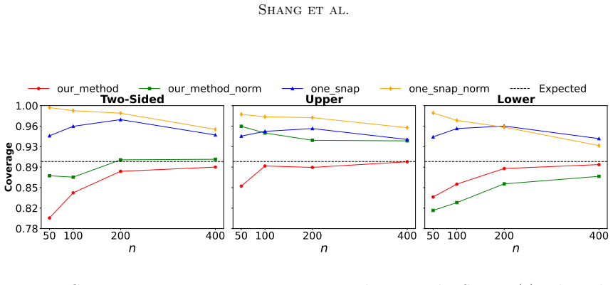
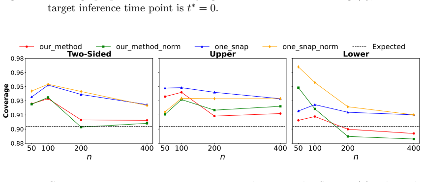
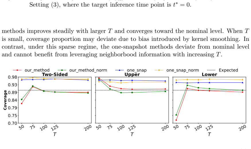
A simulation study in which the underlying graphon functions change abruptly would produce coverage rates for the studentized intervals that deviate systematically from nominal levels.
Figures


read the original abstract
Signed networks consist of both positive and negative relations, and structural balance theory provides an important conceptural framework for understanding their global tension structure. While existing statistical methods mainly focus on assessing empirical evidence of balance in a single observed network, many real-world signed relations evolve over time. This paper develops nonparametric inference for the population degree of structural balance at specified time points in dynamic signed networks, where the target time may or may not coincide with an observed snapshot. We consider a dynamic signed graphon model in which both edge formation and sign generation are governed by smoothly time-varying graphon functions. To exploit temporal smoothness, we construct a kernel-smoothed estimator that borrows information from snapshots near the target time point. Our theoretical analysis establishes a studentized inference procedure and a higher-order distributional approximation based on Edgeworth expansion, showing that temporal smoothing improves inference in sparse networks by reducing variance of observation noise, up to smoothing bias and time-discretization errors. We demonstrate the finite-sample performance and practical usefulness of the proposed method through extensive simulation studies and an application to a dynamic international relation network in political science.
Editorial analysis
A structured set of objections, weighed in public.
Referee Report
Summary. The paper develops nonparametric inference for the population degree of structural balance at target times in dynamic signed networks under a dynamic signed graphon model where edge and sign probabilities are governed by smoothly time-varying graphon functions. It constructs a kernel-smoothed estimator that borrows information across nearby snapshots, derives a studentized inference procedure, and provides a higher-order Edgeworth expansion to show that temporal smoothing reduces the variance of observation noise in sparse networks (up to smoothing bias and time-discretization errors). Finite-sample performance is assessed via simulations, and the method is applied to a dynamic international relations network.
Significance. If the theoretical results hold under the stated assumptions, the work offers a useful extension of structural balance analysis to temporal settings with explicit higher-order distributional approximations. The Edgeworth expansion and variance-reduction claim via smoothing in sparse regimes represent a technical contribution that could improve inference for evolving signed networks in applications such as political science.
major comments (2)
- [Abstract; model description paragraph] Abstract and model section: the claim that temporal smoothing improves inference by reducing variance (up to bias and discretization errors) rests on the assumption that both the edge-probability and sign-probability graphons are smooth functions of time, yet no explicit regularity index (Hölder, Sobolev, or otherwise) is supplied. Without this, it is impossible to verify that the bias term is o_p of the studentized standard deviation at the sparsity levels implicit in the signed-graphon construction, which is load-bearing for the central variance-reduction guarantee in the Edgeworth expansion.
- [Theoretical analysis (Edgeworth expansion)] Theoretical analysis section (on studentized statistic and Edgeworth expansion): the higher-order approximation is asserted to demonstrate improved inference, but the manuscript supplies no explicit verification that the smoothing bias remains negligible relative to the Edgeworth remainder under the sparsity regime. This needs to be shown with concrete rates before the studentized procedure can be guaranteed to inherit the claimed accuracy.
minor comments (1)
- [Model section] Notation for the balance measure and the two graphons (edge and sign) should be introduced with consistent symbols early in the model section to avoid ambiguity when stating the target parameter.
Simulated Author's Rebuttal
We thank the referee for the careful and constructive report. Both major comments correctly highlight the need for explicit regularity conditions and rate verifications to support the bias control underlying the variance-reduction claim. We address each point below and will revise the manuscript accordingly.
read point-by-point responses
-
Referee: [Abstract; model description paragraph] Abstract and model section: the claim that temporal smoothing improves inference by reducing variance (up to bias and discretization errors) rests on the assumption that both the edge-probability and sign-probability graphons are smooth functions of time, yet no explicit regularity index (Hölder, Sobolev, or otherwise) is supplied. Without this, it is impossible to verify that the bias term is o_p of the studentized standard deviation at the sparsity levels implicit in the signed-graphon construction, which is load-bearing for the central variance-reduction guarantee in the Edgeworth expansion.
Authors: We agree that an explicit regularity index is required to make the bias control rigorous. In the revised manuscript we will add the assumption that the time-varying edge- and sign-probability graphons belong to a Hölder class of smoothness index α > 1/2. We will then state the resulting uniform bias bound of order O(h^α) and verify, under the sparsity regime of the signed-graphon model, that this bias is o_p(σ_n) relative to the studentized scale σ_n, thereby justifying the claimed variance reduction in the Edgeworth expansion. revision: yes
-
Referee: [Theoretical analysis (Edgeworth expansion)] Theoretical analysis section (on studentized statistic and Edgeworth expansion): the higher-order approximation is asserted to demonstrate improved inference, but the manuscript supplies no explicit verification that the smoothing bias remains negligible relative to the Edgeworth remainder under the sparsity regime. This needs to be shown with concrete rates before the studentized procedure can be guaranteed to inherit the claimed accuracy.
Authors: The observation is accurate: the current text does not supply the explicit comparison of smoothing bias to the Edgeworth remainder. We will insert a new proposition (or appendix lemma) that derives the concrete rates, showing that for bandwidth sequences satisfying the usual conditions the bias term is of strictly smaller order than the Edgeworth remainder under the model’s sparsity and smoothness assumptions. This will be used to confirm that the studentized statistic inherits the stated higher-order accuracy. revision: yes
Circularity Check
No circularity detected; derivation relies on external model assumptions
full rationale
The paper develops a kernel-smoothed estimator and studentized inference procedure with Edgeworth expansion under an externally posited dynamic signed graphon model where edge and sign probabilities are governed by smoothly time-varying functions. No quoted step reduces a claimed prediction or uniqueness result to a fitted quantity, self-citation chain, or definitional tautology within the paper's own equations. The variance-reduction claim is derived from the smoothing bias-variance tradeoff under the stated Hölder-type smoothness and sparsity conditions, which are model inputs rather than outputs of the derivation. The analysis is therefore self-contained against the external graphon framework and does not exhibit any of the enumerated circularity patterns.
Axiom & Free-Parameter Ledger
axioms (1)
- domain assumption Edge formation and sign generation are governed by smoothly time-varying graphon functions.
Reference graph
Works this paper leans on
-
[1]
doi: 10.1214/15-AOS1338. Peter J. Bickel, Aiyou Chen, and Elizaveta Levina. The method of moments and degree distributions for network models.The Annals of Statistics, 39(5):2280 – 2301,
-
[2]
PJ Bickel, Friedrich G¨ otze, and WR Van Zwet
doi: 10.1214/11-AOS904. PJ Bickel, Friedrich G¨ otze, and WR Van Zwet. The edgeworth expansion for u-statistics of degree two.The Annals of Statistics, pages 1463–1484,
-
[3]
Applications of structural balance in signed social networks.arXiv preprint arXiv:1402.6865,
J´ erˆ ome Kunegis. Applications of structural balance in signed social networks.arXiv preprint arXiv:1402.6865,
-
[4]
Catherine Matias and Vincent Miele
doi: 10.1214/EJP.v12-430. Catherine Matias and Vincent Miele. Statistical clustering of temporal networks through a dynamic stochastic block model.Journal of the Royal Statistical Society Series B: Statistical Methodology, 79(4):1119–1141,
-
[5]
Warren Schudy and Maxim Sviridenko. Bernstein-like concentration and moment inequal- ities for polynomials of independent random variables: multilinear case.arXiv preprint arXiv:1109.5193,
-
[6]
Journal of the American Statistical Association , author =
doi: 10.1080/01621459.2025.2520459. Jiliang Tang, Yi Chang, Charu Aggarwal, and Huan Liu. A survey of signed network mining in social media.ACM Computing Surveys (CSUR), 49(3):1–37,
-
[7]
SinceY 1(t) = 3n−1P i g1h(Xi, t) is a sum of iid mean-zero terms, var(Y1(t)) = 9 n var(g1h(X1, t)) = 9ξ2 1h(t) n
+O(ρ 6 nn−2). SinceY 1(t) = 3n−1P i g1h(Xi, t) is a sum of iid mean-zero terms, var(Y1(t)) = 9 n var(g1h(X1, t)) = 9ξ2 1h(t) n . Lemma B.3 gives the lower boundξ 2 1h(t)≳ρ 6 n, sovar(Y 1(t))≳ρ 6 nn−1. Moreover, by Lemma B.2, it follows that var( ˜Unh(t)−U nh(t)) =O n−2(T h)−1ρ5 n +n −3(T h)−2ρ4 n +n −3(T h)−3ρ3 n . Finally, it is sufficient to compare the...
2007
-
[8]
By Lemma D.2,S K(t)≍Tand PT ℓ=1 K2 h(t−t ℓ) = O(T /h)
B.2.1 Proof of Lemma B.4 Proof.LetS K(t) = PT ℓ=1 Kh(t−t ℓ). By Lemma D.2,S K(t)≍Tand PT ℓ=1 K2 h(t−t ℓ) = O(T /h). Conditional onX, the variables{η ij(tℓ) : 1≤i < j≤n,1≤ℓ≤T}are independent, centered, and bounded. By Lemma 7.1 in Schudy and Sviridenko (2011), each ˜ηij is central moment bounded because of its boundedness. Then, Lemma D.4 could be applied ...
2011
-
[9]
The factorn −2 inµ 1q comes from the normalization n 3 −1 and theO(n) possible third vertices containing a fixed noise variable
Using| ˜Wij(t)| ≤Cρ n andE{|η ij(tℓ)| |X}= O(ρn), its hypergraph parameters satisfy µ1q =O{n −2ρ2 n(T h)−1}, µ 2q =O{n −3ρn(T h)−2}. The factorn −2 inµ 1q comes from the normalization n 3 −1 and theO(n) possible third vertices containing a fixed noise variable. By the variance bound forR q(t) and Lemma D.4, with probability at least 1−O(n −2), |Rq(t)| ≤C ...
2022
-
[10]
eisJn exp ( − s2 2nρn E[σ2 X] + 1 n nX i=1 gσ;1(Xi) !)# ds =O (nρnT h)−1 logn+n −1 logn .(S8) 32 Inference on Dynamic Signed Network It remains to bound Ψn(s) :=E
= E[g3 1h(X1, t)]√n ξ3 1h(t) + ˜Op,1(n−1 log1/2 n). Thus, the first part contributes a deterministic shift, while the off-diagonal part is a sym- metric degree-two term. For the second summand in ˇδn(t), Hoeffding decomposition gives 4 n(n−1) X i̸=j gigij ξ2 = 4 nξ2 nX i=1 ζh(Xi, t) + ˜Op,1(n−1 logn), where the first Hoeffding projection is defined as ζh(...
2001
-
[11]
The last step usesϵ ′ =ϵ/2≤1/7 and Assumption 3.4
forz=o(1), we obtain Eeis(Jn+ ˜∆n+δT ) =E[e isJn]− s2 2nρn E[eisJnσ2 X]− 1 2 cδn−1 logn s 2E[eisJn] +R G(s),(S14) where Z nϵ′ 0 RG(s) s ds≤C Z nϵ′ 0 s3E " σ2 X nρn +c δn−1 logn 2# ds =O n n4ϵ′ (nρnT h)−2 +n 4ϵ′−2 log2 n o =O{(nρ nT h)−1 +n −1 logn}. The last step usesϵ ′ =ϵ/2≤1/7 and Assumption 3.4. Next, we analyze the leading termE[e isJn] and the remai...
1972
-
[12]
Similarly, we can derive E[eisL(1) n ·isL (3) n ] 38 Inference on Dynamic Signed Network =E eisL(1) n is n3/2ξ3 1h(t) X 1≤i̸=j≤n h g1h(Xi, t){g2 1h(Xj, t)−ξ 2 1h(t)} i = is(n−1)√nξ3 1h(t) φn−2 n (s)E exp is g1h(X1, t) +g 1h(X2, t)√nξ1h(t) h g1h(X1, t){g2 1h(X2, t)−ξ 2 1h(t)} i = is(n−1)√nξ3 1h(t) φn−2 n (s))E " g1h(X1, t){g2 1h(X2, t)−ξ 2 1h(t)} +i...
2007
-
[13]
By combining the above result with (S24) and (S25), we obtain: Z nϵ′ 0 E[eis(Jn+ ˜∆n+δT )]−Ch.f.(G nh;s) s ds=O(n −1 logn+ (nρ n)−1(T h)−1)
Finally, we also have the following bound Z nϵ′ 0 E eisJn s2 2 cδn−1 logn ·s −1ds=n −1 logn·O Z nϵ′ 0 |sE[eisJn]|ds ! =O(n −1 logn), since the leading term inE[exp(isJ n)] is of the forme −t2/2P ≥0(s). By combining the above result with (S24) and (S25), we obtain: Z nϵ′ 0 E[eis(Jn+ ˜∆n+δT )]−Ch.f.(G nh;s) s ds=O(n −1 logn+ (nρ n)−1(T h)−1). Appendix D. Te...
1992
-
[14]
For the second term, sincet∈[δ,L −δ], both lower and upper limits satisfyt/h≥δ/h and (L −t)/h≥δ/h
Thus, by Lemma D.1 and Assumption 3.1, 1 h Z L 0 Kj u−t h du− 1 h X ℓ Kj tℓ −t h ∆tℓ ≤ 1 h ·T V(g; [0,L])· C T =O( 1 hT ). For the second term, sincet∈[δ,L −δ], both lower and upper limits satisfyt/h≥δ/h and (L −t)/h≥δ/h. By (K3) and|K j(u)| ≤M j−1|K(u)|, we have Z L−t h − t h Kj(u)du− Z ∞ −∞ Kj(u)du ≤ Z ∞ L−t h Kj(u) du+ Z − t h −∞ Kj(u) du ≤M j−1 Z ∞ L−...
2011
discussion (0)
Sign in with ORCID, Apple, or X to comment. Anyone can read and Pith papers without signing in.