pith. sign in

arxiv: 2606.09914 · v1 · pith:QLEEBZMQnew · submitted 2026-06-06 · 🌌 astro-ph.HE

Modelling the Dynamics of Middle-Aged Pulsar Wind Nebulae in the Reverberation Phase

Pith reviewed 2026-06-27 19:18 UTC · model grok-4.3

classification 🌌 astro-ph.HE
keywords pulsar wind nebulaereverberation phasesupernova remnantsSedov solutionhydrodynamic instabilitiesmultidimensional simulationsTeV emission
0
0 comments X

The pith

Middle-aged pulsar wind nebulae converge to a Sedov-like relaxed state despite wide diversity in their late evolution.

A machine-rendered reading of the paper's core claim, the machinery that carries it, and where it could break.

The paper models the interaction of middle-aged pulsar wind nebulae with their parent supernova remnants during the reverberation phase. It generates a synthetic population using standard distributions for pulsar and remnant parameters, then tracks evolution with a semi-analytical early phase and a 1D Lagrangian code. Despite large differences in individual tracks, every system settles into a state matching the Sedov solution for blast-wave expansion. Two-dimensional simulations show that fluid instabilities grow depending on initial conditions but leave the overall volume evolution and global dynamics essentially unchanged from the one-dimensional results. The work therefore concludes that existing one-dimensional predictions remain reliable for forecasting the long-term behavior of these nebulae.

Core claim

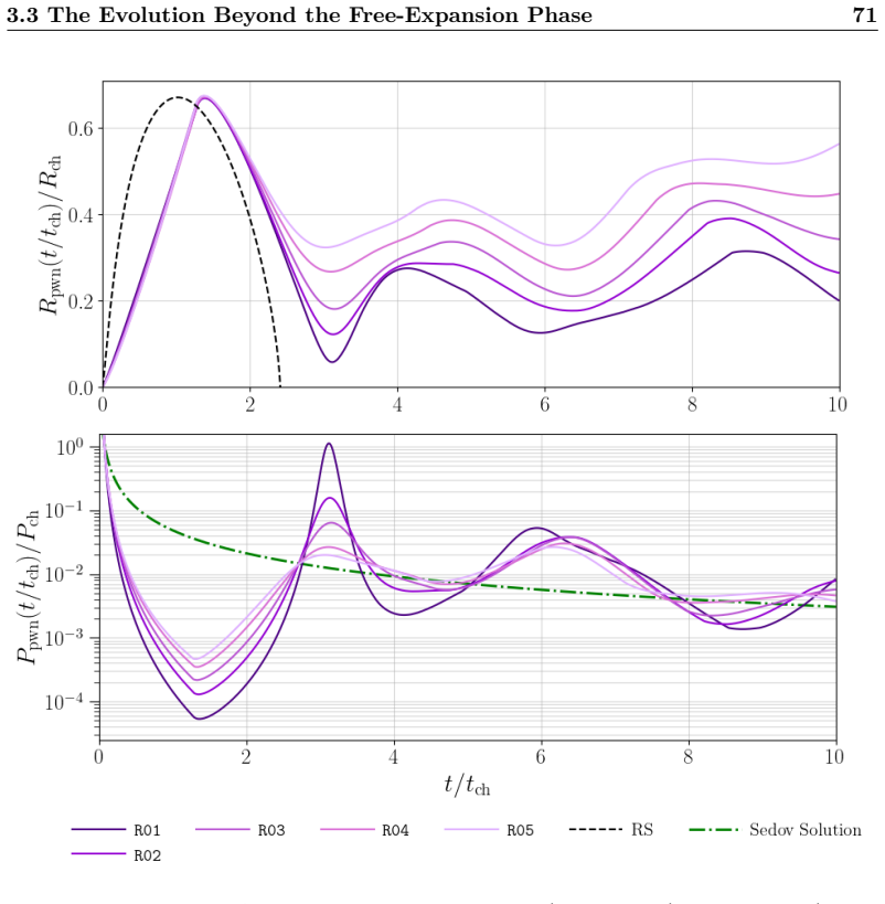
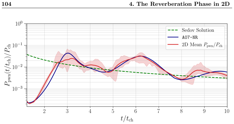
Within the region of interest that covers most synthetic systems, late-stage evolution shows substantial diversity, yet all objects converge toward a relaxed state consistent with the Sedov solution; two-dimensional simulations confirm that instability growth does not significantly alter global dynamics even though apparent size can increase by up to 50 percent.

What carries the argument

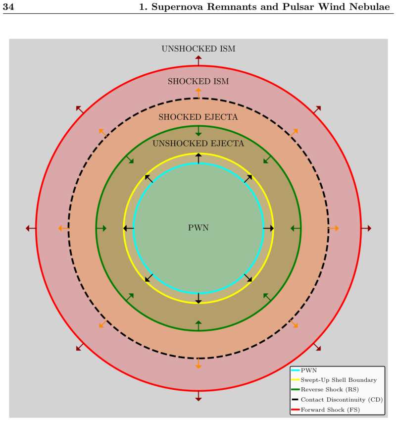
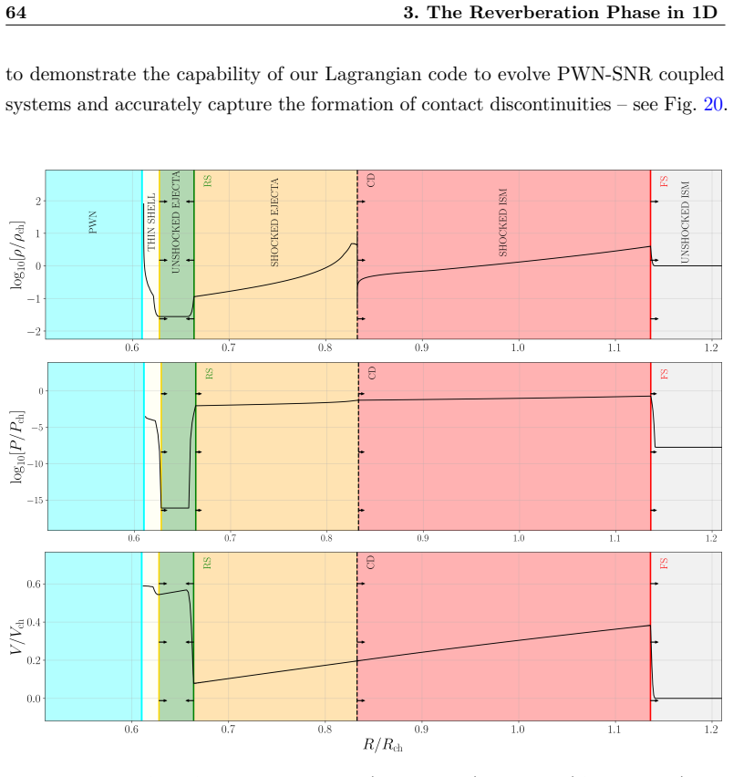
The reverberation-phase interaction between the pulsar wind nebula and the supernova remnant, tracked by a 1D Lagrangian hydrodynamics code supplemented by targeted 2D simulations that preserve physical accuracy while limiting cost.

If this is right

  • One-dimensional models can be used with confidence to predict the late-time size and energy content of the majority of Galactic TeV-emitting PWNe.
  • Population synthesis studies of middle-aged PWNe no longer need to treat multidimensional mixing as a dominant source of uncertainty in global quantities.
  • The Sedov-like endpoint provides a simple analytic anchor for estimating the contribution of these nebulae to the diffuse Galactic gamma-ray background.
  • Future high-energy observatories can rely on existing one-dimensional evolutionary tracks when planning surveys of middle-aged PWNe.

Where Pith is reading between the lines

These are editorial extensions of the paper, not claims the author makes directly.

  • If the Sedov convergence holds across the observed population, then the scatter in measured PWN sizes at a given age should be dominated by initial conditions rather than by late-time instabilities.
  • The reported 50 percent increase in apparent size suggests that resolved imaging of individual objects may reveal larger extents than one-dimensional models predict, offering a testable signature in radio or X-ray maps.
  • Because the result is obtained for a representative synthetic population, extending the same parameter scan to lower or higher ambient densities would map the boundaries of the region where convergence still occurs.

Load-bearing premise

Two-dimensional simulations optimized for computational efficiency are still sufficient to show that instabilities leave global dynamics unchanged.

What would settle it

A direct measurement showing that the observed radius or volume evolution of a middle-aged PWN deviates systematically from the one-dimensional prediction by more than the 50 percent margin allowed by multidimensional mixing.

Figures

Figures reproduced from arXiv: 2606.09914 by Niccol\`o Bucciantini, Yuri Batini.

Figure 1
Figure 1. Figure 1: Upper panels: old PWNe observed by HESS in the TeV band. From left to right: Vela X, HESS J1420-607 & HESS J1418-609, and HESS J1825–137. The color scale represents the excess of TeV emission with respect to the background in arbitrary units (Aharonian et al. 2006b, Aharonian et al. 2006c, Aharonian et al. 2006e. Bottom panels: SNR G320.4-1.2 with the inner, young PWN observed in the X-rays by Chandra (Lef… view at source ↗
Figure 2
Figure 2. Figure 2: Left panel: schematic representations of a spherically symmetric SNR by Reynolds (2017). Right panel: density profile of a SNR expanding in the ISM by Bandiera et al. (2021), characterized by a core (R ≤ Rcore) and an envelope (Rcore < R ≤ Renv). We anticipate that the density of the cold ejecta scales as r −δ – with δ ≃ 0 – in the core, and as r −ω – with ω ≃ 12 – in the envelope (Matzner & McKee, 1999). … view at source ↗
Figure 3
Figure 3. Figure 3: SNRs observed in X-rays by Chandra. Left panel: G1.9+0.3 (associated with a SN dating to ≃ 1900 AD). Center panel: Kepler SNR G4.5+6.8 (associated with SN 1604). Right panel: Tycho SNR G120.1+1.4 (associated with SN 1572). of this phase are X-rays and recombination continuum. As the FS decelerates down to ≃ 200 km s−1 , eventually the characteristic cooling time of the gas (which depends on its chemical co… view at source ↗
Figure 4
Figure 4. Figure 4: The evolutionary path of the RS inside a SNR for δ = 0 and ω = 12 (Bandiera et al., 2021). time tmin, given by: tmin ≃ 2.5tch ≃ 8100  Esn 1051 erg− 1 2  Mej 10M⊙  5 6 " m0n0 mpcm−3 #− 1 3 yrs. (1.21) Once the RS has reached the center of the SNR, all the ejecta have been re-heated and the SNR relaxes into a fully self-similar state, where the radius of the FS evolves as RFS ∝ t 2/5 , according to the S… view at source ↗
Figure 5
Figure 5. Figure 5: Schematical representation of the magnetosphere of a NS. µns represents the magnetic dipole moment of the NS and Ωns its rotational axis. The vertical dashed lines mark the light cylinder radius RLC. Green lines represent the closed magnetic field lines, extended within RLC. On the contrary, red lines represent magnetic field lines extending beyond RLC. into account the geometry of the dipolar magnetic fie… view at source ↗
Figure 6
Figure 6. Figure 6: Images of the Crab Nebula in different bands. Upper-left panel: Radio (VLA)5 . Upper-right panel: Infrared (Spitzer)5 . Lower-left panel: Optical (HST)5 . Lower-right panel: X-rays (Chandra)6 . Note that panels are not in scale to each other; the radio, infrared and optical regions are significantly larger than the X-ray. 1.3.2 Models of Pulsar Wind Nebulae In this section we will present a simplified mode… view at source ↗
Figure 7
Figure 7. Figure 7: Spectral energy distribution of the Crab Nebula, comparing observational data with the best-fit model (green line, Dirson & Horns 2023). The model sums thermal dust emission with the synchrotron and IC radiation produced by two distinct electron populations: radio (R) and wind (W) electrons. The bottom panel shows the relative residuals. ejecta with continuum emission from dust, condensed from the cold eje… view at source ↗
Figure 8
Figure 8. Figure 8: Schematic representation of a spherically symmetric PWN expanding in the parent SNR. (Slane 2017, Abeysekara et al. 2020a). In the end, since pulsars typically possess high birth kick velocities (Vpsr ≃ 300km s−1 , Hansen & Phinney 1997) the central source is expected to eventually leave the parent SNR. Equating the displacement of the PSR with the radius of the SNR in the Sedov phase, yields the typical e… view at source ↗
Figure 9
Figure 9. Figure 9: Normalized histograms of the distributions of L0 and τ0 for a young population of 104 PSRs. Remarkably, the majority of the population exhibits initial spin-down luminosities ≃ 1038 erg s−1 and initial spin-down timescales ≃ 5 kyr. In [PITH_FULL_IMAGE:figures/full_fig_p052_9.png] view at source ↗
Figure 10
Figure 10. Figure 10: Diagram of the period derivative vs period for both observed and synthetic PSRs. For the synthetic population we report the initial period and its derivative, whereas for the observed Galactic population we plot the current values. The dashed diagonal lines represent configurations of constant magnetic field, calculated using Eq. (1.28). Among the deteced PSRs we identify three main populations: canonical… view at source ↗
Figure 11
Figure 11. Figure 11: Normalized histograms of the distributions of Lch, tch and Rch for a population of 104 SNRs. in the range [5 − 50] pc and peaks at Rch ≃ 15pc. We recall that these scales, together with the characteristic velocity and pressure – Vch and Pch – given by Eq. (1.7) and Eq. (1.11), govern the dynamical evolution of SNRs. We remark that a single characteristic scale does not uniquely identify a single progenito… view at source ↗
Figure 12
Figure 12. Figure 12: PDF of the PWN-SNR synthetic population in the characteristic plane, with the colorbar indicating its values. While the external, thin ellipse encloses the entire sample, the inner, thick boundary encloses 95 % of the population, and defines our ROI. enclosed by the inner boundary in [PITH_FULL_IMAGE:figures/full_fig_p058_12.png] view at source ↗
Figure 13
Figure 13. Figure 13: Distribution of trev/tch within the ROI. The color gradient indicates the magnitude of the variable. The smooth internal contours trace the isolines of the quantity, uniformly spaced from its minimum to its maximum value. with higher velocities – typically ≳ Vch – larger swept-up masses (≳ 0.3Mej) – and higher internal pressure (≳ 10−2Pch) than the fainter ones, despite exhibiting similar radii, ≃ [0.3 − … view at source ↗
Figure 14
Figure 14. Figure 14: Distributions of Rpwn(trev/tch)/Rch, Ppwn(trev/tch)/Pch, Msh(trev/tch)/Mej and Vpwn(trev/tch)/Vch within the ROI. The smooth internal contours trace the isolines uniformly spaced from the minimum to the maximum value. energetic budget as: Esd ≡ Z ∞ 0 Lsd(t)dt, (2.14) we identify: Einj(trev) ≡ Z trev 0 Lsd(t)dt and Eava(trev) ≡ Z ∞ trev Lsd(t)dt. (2.15) Note that Einj(trev) + Eava(trev) = Esd. Evidently, t… view at source ↗
Figure 15
Figure 15. Figure 15: Distributions of Esh(trev/tch)/Esn, Epwn(trev/tch)/Esn, Einj(trev/tch)/Esn and Eava(trev/tch)/Esn within the ROI. The smooth internal contours trace the isolines uniformly spaced from the minimum to the maximum value. injection – Einj ≃ 10−5Esn. Regarding the internal energy, although more pow￾erful systems exhibit higher values at the beginning of the reverberation phase, this component remains significa… view at source ↗
Figure 16
Figure 16. Figure 16: Relation between the zero age main sequence mass of the progenitor – M – and the stellar mass just before the SN explosion occurs – MPre−SN. While the black dots represents the results of Sukhbold et al. (2016), the red, solid line represents the best-fit function, obtained using a 5th-order polynomial [PITH_FULL_IMAGE:figures/full_fig_p063_16.png] view at source ↗
Figure 17
Figure 17. Figure 17: Cumulative distribution function of the density at the site of the SN explosion for varying numerical resolution (fSN representing cumulative fraction of SNe in regions where the ambient density is smaller than n0 (Kim & Ostriker, 2017)). Upper panel: SNe explosions occurring in clusters (subsctipt cl). Lower panel: SNe explosions of runaway stars (subscript run) [PITH_FULL_IMAGE:figures/full_fig_p065_17.png] view at source ↗
Figure 18
Figure 18. Figure 18: Comparison between the canonical ROI, derived in Sect. 2.3 (black) and the region obtained by accounting for the mass loss of the progenitor (Sukhbold et al., 2016) and the sampling of the ISM given by Kim & Ostriker (2017) (red) [PITH_FULL_IMAGE:figures/full_fig_p066_18.png] view at source ↗
Figure 19
Figure 19. Figure 19: Groups of systems sampled across the ROI (red solid line), along the major axis (A, Upper-left panel), in the same isolevel of trev/tch (R, Upper-right panel), at fixed τ0/tch (T, Lower-left panel) and L0/Lch (L, Lower-right panel), see also Table (3.1). System log10[τ0/tch] log10[L0/Lch] CF System log10[τ0/tch] log10[L0/Lch] CF A01 −1.59 0.74 1.81 R01 −1.02 −1.75 11.1 A02 −1.47 0.21 2.27 R02 −0.51 −2.07 … view at source ↗
Figure 20
Figure 20. Figure 20: Profiles of normalized density (Upper panel), pressure (Center panel) and velocity (Lower panel), extending from the boundary of the PWN to the ISM for the class of equivalent systems A07, evaluated at t = 1.1tch, reproducing the schematical representation in [PITH_FULL_IMAGE:figures/full_fig_p072_20.png] view at source ↗
Figure 21
Figure 21. Figure 21: Evolution of the normalized density (Upper panel), pressure (Center panel), and velocity (Lower panel) for the case A07. It is possible to distinguish the PWN (black area in the density graphics), the RS, the CD, the RS and the Thin-Shell (TS). Several shocks are produced as contact discontinuities interact. Among these, we recognize the PWN compression shock (PWNCS), the Transmitted Secondary Shock (TSS)… view at source ↗
Figure 22
Figure 22. Figure 22: Evolution of the normalized nebular radius (Upper panel) and pressure (Lower panel) for the PWN-SNR systems sampled along the major axis of the ROI (group A). initial free-expansion phase. As a consequence, the observational probability of de￾tecting a PWN that has already undergone the collision with the RS is considerably higher than finding one in the free-expansion stage, provided its residual luminos… view at source ↗
Figure 23
Figure 23. Figure 23: Evolution of the normalized nebular radius (Upper panel) and pressure (Lower panel) for the PWN-SNR systems with the same normalized reverberation time (group R). differences in terms of radial profile. It is noteworthy, however, that all systems reach the minimum radii simultaneously at ≃ 3tch and at ≃ 6tch. In agreement with our previous findings, systems possessing larger energy reserves exhibit lower … view at source ↗
Figure 24
Figure 24. Figure 24: Evolution of the normalized nebular radius (Upper panel) and pressure (Lower panel) for the PWN-SNR systems with identical initial spin-down time (group T). of groups R and A. Despite this temporal and dynamical heterogeneity, the systems once again exhibit a remarkable convergence in their final states of pressure. By the end of the simulation, the dispersion of the pressure is minimal, settling within t… view at source ↗
Figure 25
Figure 25. Figure 25: Evolution of the normalized nebular radius (Upper panel) and pressure (Lower panel) for the PWN-SNR systems with identical initial spin-down luminosity (group L). Recalling the findings presented in Sect. 2.4 and Figs. 14– 15, although these systems arrive at the reverberation phase with a comparable energy injection from the PSR, they possess vastly different energy budgets available to sustain the subse… view at source ↗
Figure 26
Figure 26. Figure 26: Mean pressure (black solid line) obtained by the evolution of the models reported in [PITH_FULL_IMAGE:figures/full_fig_p084_26.png] view at source ↗
Figure 27
Figure 27. Figure 27: The termination shock of the PSR wind for the system A07. For this specific case, τ0/tch ≃ 0.50, L0/Lch ≃ 8.9 × 10⁻³ , and Vch/c ≃ 7.3 × 10⁻³ . Comparing [PITH_FULL_IMAGE:figures/full_fig_p088_27.png] view at source ↗
Figure 28
Figure 28. Figure 28: Evolution of the normalized nebular radius (Upper panel) and pressure (Lower panel) for the PWN-SNR systems A07 and its non-relativistic counterpart, without energy injection from the central PSR (A07-NR). The two systems obviously share identical profiles both of radius and pressure during the free-expansion phase up to the compression, and their subsequent evolution is quite similar, with minor quantita… view at source ↗
Figure 29
Figure 29. Figure 29: Evolution of the normalized density (Upper panel), pressure (Center panel), and velocity (Lower panel) for the system A07-NR. It is possible to distinguish the PWN (black area in the density plot), the RS, the CD, the FS and the Thin-Shell (TS). Several shocks are produced as contact discontinuities interact. Among these, we recognize the PWN compression shock (PWNCS), the Transmitted Secondary Shock (TSS… view at source ↗
Figure 30
Figure 30. Figure 30: Profiles of density (Upper panel) and velocity (Lower panel) in the case ρpwn = 5Ppwnc −2 and ρpwn = 50Ppwnc −2 at ≃ 3tch, during maximum compression. While the RS has been dissolved by the interaction with the Thin Swept-Up Shell (TS) – here located between ≃ 0.23Rch and 0.27Rch – it is still possible to identify the CD and the FS, located at ≃ 0.9Rch and ≃ 1.8Rch, respectively. across all levels – a sta… view at source ↗
Figure 31
Figure 31. Figure 31: Initial 2D density map of the A07-NR PWN-SNR system, with amplitude perturbation η = 0.30 and wavenumber nθ = 2. From the center outward: the PWN (blue area), the thin perturbed swept-up shell, unshocked ejecta, RS, shocked ejecta, CD, shocked ISM, FS, followed by the unshocked ISM. Radial Boundary Conditions At the inner boundary – Rmin – we impose a radial reflective condition. In this regime, pressure,… view at source ↗
Figure 32
Figure 32. Figure 32: Time evolution of log10[ρ/ρch] during the compression phase of the PWN, with an initial perturbation amplitude η = 0.30 and an angular wavenumber nθ = 2. develop in the PWN, close to the boundary itself, with convective motions converg￾ing toward the regions with over-density. This vorticity drives the growth of the Kelvin-Helmholtz instability at the interface that, together with shear instabilities, cau… view at source ↗
Figure 33
Figure 33. Figure 33: log10[ρ/ρch] during the compression phase of the PWN, at η = 0.3 and t = 1.6tch. By maintaining a fixed amplitude of the perturbation – η = 0.30 – it becomes evident that increasing the angular wavenumber nθ significantly anticipates the development of the instabilities. Notably, while the trailing over-dense regions maintain a characteristic mass density of ≃ 0.1ρch across all analyzed models, the densit… view at source ↗
Figure 34
Figure 34. Figure 34: log10[ρ/ρch] during the compression phase of the PWN, at nθ = 4 and t = 1.6tch. with the weakest perturbation – η = 0.05 – the evolution is notably delayed, with only the trailing over-dense regions between 0.60Rch and 0.65Rch. As the amplitude is increased to η = 0.10, the penetration fingers begin to emerge, approximately extending from ≃ 0.60Rch to ≃ 0.62Rch and exhibiting an internal mass density of ≃… view at source ↗
Figure 35
Figure 35. Figure 35: log10[ρ/ρch] during the compression phase of the PWN, at η = 0.30 and t = 2.0tch. The trend that we have previously established regarding the faster onset of the instability at higher wavenumbers – observed in [PITH_FULL_IMAGE:figures/full_fig_p103_35.png] view at source ↗
Figure 36
Figure 36. Figure 36: log10[ρ/ρch] during the compression phase of the PWN, at nθ = 4 and t = 2.0tch. developed. Despite this, the formation of penetration fingers – with a characteristic density of ≃ 10−3ρch – is evident, anchored by a dense base – where ρ ≃ 0.1ρch. Combined, these fingers and their base extend from ≃ 0.44Rch to ≃ 0.46Rch. The trailing over-densities – which maintain a characteristic density of ≃ 0.1ρch acros… view at source ↗
Figure 37
Figure 37. Figure 37: log10[ρ/ρch] during the compression phase of the PWN, at η = 0.30 and t = 2.5tch. ≃ 0.37Rch. Finally, the nθ = 4 model shows the compression in a far more advanced state and in this latter scenario, the bounce shock is slightly advanced compared to the previous cases. In this case, the bounce shock is destined to propagate through a region where the over-densities are significantly more frayed – although … view at source ↗
Figure 38
Figure 38. Figure 38: log10[ρ/ρch] during the compression phase of the PWN, at nθ = 4 and t = 2.5tch. and they exhibit some turbulent mixing. Furthermore, the over-dense regions above the nebula extend from ≃ 0.30Rch to ≃ 0.40Rch both in the η = 0.05 and η = 0.10 case, their global density is ≃ 0.1ρch and their structure is well-defined. Notably, the internal unmixed structure of the nebula is significantly broader for η = 0.0… view at source ↗
Figure 39
Figure 39. Figure 39: Time evolution of log10[ρ/ρch] after the compression, with an initial perturbation amplitude η = 0.30 and an angular wavenumber nθ = 4. As the nebula re-expands, reaches a maximum radius of ≃ 0.40Rch at 5tch – see panel B. By this time, the bounce shock has reached the CD at ≃ 0.75Rch. This interaction generates both a reflected shock and a transmitted shock, the latter of which carries outward the pertur… view at source ↗
Figure 40
Figure 40. Figure 40: Evolution of the internal pressure of the PWN. The thick, blue solid line represents the 1D non-relativistic case A07-NR, while the red line indicates the average pressure derived from the profiles sampled at various points within the PWN, with the shaded transparent band encompassing all the pressure profiles extracted across the selected points. The green, dashed line representing the Sedov solution. at… view at source ↗
Figure 41
Figure 41. Figure 41: Density of the PWN material at t = 9.0 tch in the case with amplitude η = 0.30 and wavenumber nθ = 4. Up to ≃ 0.30Rch, the density of the PWN material looks pretty uniform in distri￾bution. Beyond this radius, mixing is evident. At radii ≳ 0.40Rch bubbles of PWN material embedded into the SNR material are present, extending up to ≃ 0.70Rch. There is some indication that bubbles present at the edge around … view at source ↗
Figure 42
Figure 42. Figure 42: Comparison among the radius of the 1D case A07-NR (blue solid line), the mean effective radius (red solid line), and the mean apparent radius (yellow solid line). The yellow and red shaded transparent bands encompass all the effective and apparent radial profiles in the cases with nθ = 4, with varying η. Consistent with the findings from the average pressure of the nebula, the effec￾tive radius R (eff) pw… view at source ↗
Figure 43
Figure 43. Figure 43: Simulated data (blue) and associated PDFs (red lines) for the physical quantities discussed above [PITH_FULL_IMAGE:figures/full_fig_p120_43.png] view at source ↗
Figure 44
Figure 44. Figure 44: Evolution of the normalized density (Upper panel), pressure (Center panel), and velocity (Lower panel) for the system T01 [PITH_FULL_IMAGE:figures/full_fig_p124_44.png] view at source ↗
Figure 45
Figure 45. Figure 45: Evolution of the normalized density (Upper panel), pressure (Center panel), and velocity (Lower panel) for the system L05 [PITH_FULL_IMAGE:figures/full_fig_p125_45.png] view at source ↗
read the original abstract

Pulsar Wind Nebulae (PWNe) are among the most important sources emitting in the very-high-energy gamma-ray band. Predicting their long-term evolution is crucial for forthcoming high-energy observatories like ASTRI and CTA. In this work, We investigate the dynamical evolution of middle-aged PWNe - probably the major contributors to the Galactic TeV emission - and test the robustness of current approaches. To understand the diversity of these systems, we derive the Pulsar and Supernova Remnant (SNR) parameters governing PWN evolution. SNR evolution is set by supernova kinetic energy, ejecta mass, and ambient density, while pulsar energy injection powers the PWN expansion. Adopting standard distributions, we generate a synthetic PWN-SNR population and define a region of interest encompassing the majority of these objects. We use a semi-analytical framework for the early evolution and a 1D Lagrangian code to track their interaction with parent SNRs (the reverberation phase). Within our region of interest, we find large diversity in the late-stage evolution. Despite this, all systems converge toward a relaxed state consistent with the Sedov solution. To address 1D limitations, we perform 2D simulations - optimized to reduce computational cost while preserving physical accuracy - to study instability growth and long-term mixing. We find that instability growth depends on initial perturbations but does not significantly alter global dynamics. While effective volume evolution agrees with 1D predictions, multidimensional effects can increase the apparent size by up to 50%. For the first time, we investigated in detail the multidimensional evolution of middle-aged PWNe in the reverberation phase. By characterizing the late-time evolution across the population, our results confirm the robustness of 1D models, demonstrating that current predictions remain trustworthy.

Editorial analysis

A structured set of objections, weighed in public.

Desk editor's note, referee report, simulated authors' rebuttal, and a circularity audit. Tearing a paper down is the easy half of reading it; the pith above is the substance, this is the friction.

Referee Report

1 major / 1 minor

Summary. The paper models the long-term dynamical evolution of middle-aged pulsar wind nebulae (PWNe) in the reverberation phase. Using a synthetic population drawn from standard distributions of supernova and pulsar parameters, it employs semi-analytical methods for early phases and 1D Lagrangian hydrodynamics for the interaction with the parent SNR. Despite large diversity in late-stage behavior, all models converge to a relaxed state consistent with the Sedov solution. 2D simulations (optimized for computational cost) are used to assess instability growth; the authors conclude that multidimensional effects do not significantly alter global dynamics, thereby confirming the robustness of 1D predictions, while noting that apparent sizes can increase by up to 50%.

Significance. If the central claims hold, the work provides a useful population-level characterization of middle-aged PWNe relevant to TeV emission predictions for CTA and ASTRI. The synthetic population generation, explicit mapping of governing parameters (supernova kinetic energy, ejecta mass, ambient density, pulsar injection rate), and direct benchmarking of 1D results against the independent Sedov solution are strengths. The attempt to quantify multidimensional corrections to 1D models addresses a recognized limitation in the field.

major comments (1)
  1. [Abstract and 2D simulations section] Abstract (paragraph on 2D simulations) and corresponding methods/results section: the claim that 'instability growth does not significantly alter global dynamics' and that 2D results 'confirm the robustness of 1D predictions' rests on simulations described only as 'optimized to reduce computational cost while preserving physical accuracy.' No grid resolution, domain size, perturbation amplitude, or convergence metrics are reported for the reverberation-phase contact discontinuity. Without these, it is impossible to determine whether the reported agreement with 1D radius evolution and Sedov convergence is robust or an artifact of numerical suppression of Rayleigh-Taylor/Kelvin-Helmholtz mixing, especially across the noted diversity of late-stage evolutionary tracks.
minor comments (1)
  1. [Abstract] Abstract: the sentence 'In this work, We investigate...' contains an unnecessary capital 'W' in 'We'.

Simulated Author's Rebuttal

1 responses · 0 unresolved

We thank the referee for their constructive report and recommendation. We address the single major comment below.

read point-by-point responses
  1. Referee: [Abstract and 2D simulations section] Abstract (paragraph on 2D simulations) and corresponding methods/results section: the claim that 'instability growth does not significantly alter global dynamics' and that 2D results 'confirm the robustness of 1D predictions' rests on simulations described only as 'optimized to reduce computational cost while preserving physical accuracy.' No grid resolution, domain size, perturbation amplitude, or convergence metrics are reported for the reverberation-phase contact discontinuity. Without these, it is impossible to determine whether the reported agreement with 1D radius evolution and Sedov convergence is robust or an artifact of numerical suppression of Rayleigh-Taylor/Kelvin-Helmholtz mixing, especially across the noted diversity of late-stage evolutionary tracks.

    Authors: We agree that the current manuscript lacks the quantitative numerical details needed to allow independent evaluation of the 2D results. In the revised manuscript we will add a dedicated subsection describing the 2D setup, including: (i) the grid resolution and any adaptive refinement strategy employed at the contact discontinuity, (ii) the size of the computational domain relative to the PWN radius, (iii) the amplitude and spectrum of the initial perturbations used to seed Rayleigh-Taylor and Kelvin-Helmholtz instabilities, and (iv) the outcome of resolution and domain-size convergence tests performed on representative reverberation-phase models. These additions will be cross-referenced to the abstract claim and will explicitly address whether the reported 50 % increase in apparent size and the preservation of global 1D-like dynamics remain robust across the diversity of late-stage tracks. revision: yes

Circularity Check

0 steps flagged

No circularity; forward simulations benchmarked to independent Sedov solution

full rationale

The derivation relies on standard input distributions for SNR/PWN parameters, a semi-analytical early-phase model, a 1D Lagrangian hydro code, and 2D simulations whose global outputs are compared directly to the external Sedov solution. No fitted parameter is renamed as a prediction, no self-citation supplies a load-bearing uniqueness theorem or ansatz, and the central claim of convergence plus limited multidimensional impact is not forced by construction from the paper's own inputs. The chain is self-contained against external benchmarks.

Axiom & Free-Parameter Ledger

4 free parameters · 2 axioms · 0 invented entities

The modeling framework draws supernova and pulsar parameters from standard literature distributions without fitting new constants to the target data; relies on established hydrodynamic equations and the Sedov solution as external benchmarks.

free parameters (4)
  • supernova kinetic energy
    Drawn from standard distributions to generate synthetic PWN-SNR population
  • ejecta mass
    Drawn from standard distributions to generate synthetic PWN-SNR population
  • ambient density
    Drawn from standard distributions to generate synthetic PWN-SNR population
  • pulsar energy injection rate
    Powers PWN expansion; taken from pulsar parameter distributions
axioms (2)
  • standard math Standard hydrodynamic equations govern PWN-SNR interaction
    Implemented in the 1D Lagrangian code for reverberation phase
  • standard math Late-time evolution follows the Sedov blast-wave solution
    Used as benchmark for the relaxed state reached by all simulated systems

pith-pipeline@v0.9.1-grok · 5860 in / 1504 out tokens · 33144 ms · 2026-06-27T19:18:26.189496+00:00 · methodology

discussion (0)

Sign in with ORCID, Apple, or X to comment. Anyone can read and Pith papers without signing in.

Reference graph

Works this paper leans on

188 extracted references · 177 canonical work pages · 7 internal anchors

  1. [1]

    Abdalla H., et al., 2021, @doi [Science] 10.1126/science.abe8560 , 372, 1081–1085

  2. [2]

    U., et al., 2017, @doi [Science] 10.1126/science.aan4880 , https://ui.adsabs.harvard.edu/abs/2017Sci...358..911A 358, 911

    Abeysekara A. U., et al., 2017, @doi [Science] 10.1126/science.aan4880 , https://ui.adsabs.harvard.edu/abs/2017Sci...358..911A 358, 911

  3. [3]

    U., et al., 2018, @doi [ ] 10.3847/1538-4357/aade4e , 866, 24

    Abeysekara A. U., et al., 2018, @doi [ ] 10.3847/1538-4357/aade4e , 866, 24

  4. [4]

    Abeysekara A., et al., 2020a, @doi [Astroparticle Physics] https://doi.org/10.1016/j.astropartphys.2019.102403 , 117, 102403

  5. [5]

    U., et al., 2020b, @doi [ ] 10.1103/PhysRevLett.124.021102 , https://ui.adsabs.harvard.edu/abs/2020PhRvL.124b1102A 124, 021102

    Abeysekara A. U., et al., 2020b, @doi [ ] 10.1103/PhysRevLett.124.021102 , https://ui.adsabs.harvard.edu/abs/2020PhRvL.124b1102A 124, 021102

  6. [6]

    S., et al., 2018, Science with the Cherenkov Telescope Array

    Acharya B. S., et al., 2018, Science with the Cherenkov Telescope Array . WSP, @doi 10.1142/10986

  7. [7]

    Aharonian F., et al., 2001, @doi [ ] 10.1051/0004-6361:20010243 , https://ui.adsabs.harvard.edu/abs/2001A&A...370..112A 370, 112

  8. [8]

    Aharonian F., et al., 2004, @doi [ ] 10.1038/nature02960 , https://ui.adsabs.harvard.edu/abs/2004Natur.432...75A 432, 75

  9. [9]

    Aharonian F., et al., 2005, @doi [ ] 10.1051/0004-6361:200500105 , 435, L17–L20

  10. [10]

    Aharonian F., et al., 2006a, @doi [PRL] 10.1103/PhysRevLett.97.221102 , https://ui.adsabs.harvard.edu/abs/2006PhRvL..97v1102A 97, 221102

  11. [11]

    Aharonian F., et al., 2006b, @doi [ ] 10.1051/0004-6361:200600014 , https://ui.adsabs.harvard.edu/abs/2006A&A...448L..43A 448, L43

  12. [12]

    Aharonian F., et al., 2006c, @doi [ ] 10.1051/0004-6361:20065511 , 456, 245–251

  13. [13]

    Aharonian F., et al., 2006d, @doi [ ] 10.1051/0004-6361:20065351 , https://ui.adsabs.harvard.edu/abs/2006A&A...457..899A 457, 899

  14. [14]

    Aharonian F., et al., 2006e, @doi [ ] 10.1051/0004-6361:20065546 , 460, 365–374

  15. [15]

    A., Cheng A

    Alpar M. A., Cheng A. F., Ruderman M. A., Shaham J., 1982, @doi [ ] 10.1038/300728a0 , https://ui.adsabs.harvard.edu/abs/1982Natur.300..728A 300, 728

  16. [16]

    W., Murdin P., 2017, in Alsabti A

    Alsabti A. W., Murdin P., 2017, in Alsabti A. W., Murdin P., eds, , Handbook of Supernovae. p. 3, @doi 10.1007/978-3-319-21846-5_1

  17. [17]

    B., et al., 2009, @doi [ ] 10.1088/0004-637x/697/2/1071 , 697, 1071–1102

    Atwood W. B., et al., 2009, @doi [ ] 10.1088/0004-637x/697/2/1071 , 697, 1071–1102

  18. [18]

    Baade W., Zwicky F., 1934, @doi [Proceedings of the National Academy of Sciences] 10.1073/pnas.20.5.259 , 20, 259

  19. [19]

    Backer D., Kulkarni S., Heiles C., Davis M., Goss M., 1982, , https://ui.adsabs.harvard.edu/abs/1982IAUC.3743....2B 3743, 2

  20. [20]

    F., 2020, @doi [ ] 10.1093/mnras/staa2956 , https://ui.adsabs.harvard.edu/abs/2020MNRAS.499.2051B 499, 2051

    Bandiera R., Bucciantini N., Mart \' n J., Olmi B., Torres D. F., 2020, @doi [ ] 10.1093/mnras/staa2956 , https://ui.adsabs.harvard.edu/abs/2020MNRAS.499.2051B 499, 2051

  21. [21]

    F., 2021, @doi [ ] 10.1093/mnras/stab2600 , https://ui.adsabs.harvard.edu/abs/2021MNRAS.508.3194B 508, 3194

    Bandiera R., Bucciantini N., Mart \' n J., Olmi B., Torres D. F., 2021, @doi [ ] 10.1093/mnras/stab2600 , https://ui.adsabs.harvard.edu/abs/2021MNRAS.508.3194B 508, 3194

  22. [22]

    F., 2023a, @doi [ ] 10.1093/mnras/stad134 , 520, 2451–2472

    Bandiera R., Bucciantini N., Martín J., Olmi B., Torres D. F., 2023a, @doi [ ] 10.1093/mnras/stad134 , 520, 2451–2472

  23. [23]

    F., 2023b, @doi [ ] 10.1093/mnras/stad2387 , 525, 2839–2850

    Bandiera R., Bucciantini N., Olmi B., Torres D. F., 2023b, @doi [ ] 10.1093/mnras/stad2387 , 525, 2839–2850

  24. [24]

    G., 2011, in Torres D

    Baring M. G., 2011, in Torres D. F., Rea N., eds, Astrophysics and Space Science Proceedings Vol. 21, High-Energy Emission from Pulsars and their Systems. p. 453, @doi 10.1007/978-3-642-17251-9_38

  25. [25]

    A., Pizzochero P., 1990, @doi [ ] 10.1086/185661 , https://ui.adsabs.harvard.edu/abs/1990ApJ...350L..33B 350, L33

    Bethe H. A., Pizzochero P., 1990, @doi [ ] 10.1086/185661 , https://ui.adsabs.harvard.edu/abs/1990ApJ...350L..33B 350, L33

  26. [26]

    Biswas B., Rosswog S., 2025, @doi [ ] 10.1103/8lv3-1ywb , https://ui.adsabs.harvard.edu/abs/2025PhRvD.112b3045B 112, 023045

  27. [27]

    M., Chevalier R

    Blondin J. M., Chevalier R. A., Frierson D. M., 2001, @doi [ ] 10.1086/324042 , https://ui.adsabs.harvard.edu/abs/2001ApJ...563..806B 563, 806

  28. [28]

    On the physics of cold MHD winds from oblique rotators

    Bogovalov S. V., 1999, @doi [ ] 10.48550/arXiv.astro-ph/9907051 , https://ui.adsabs.harvard.edu/abs/1999A&A...349.1017B 349, 1017

  29. [29]

    Bombaci Popov 2004, @doi [A&A] 10.1051/0004-6361:20041142 , 424, 627

  30. [30]

    Bonollo A., Esposito P., Giuliani A., Caraveo P., Galanti G., Crestan S., Rigoselli M., Mereghetti S., 2026, @doi [Journal of High Energy Astrophysics] 10.1016/j.jheap.2025.100465 , 50, 100465

  31. [31]

    Borwankar S., et al., 2024, @doi [Astroparticle Physics] 10.1016/j.astropartphys.2024.102960 , 159, 102960

  32. [32]

    Bosch-Ramon V., 2006, in VI Microquasar Workshop: Microquasars and Beyond. p. 5.1, @doi 10.22323/1.033.0005

  33. [33]

    T., Chubb T

    Bowyer S., Byram E. T., Chubb T. A., Friedman H., 1964, @doi [Science] 10.1126/science.146.3646.912 , https://ui.adsabs.harvard.edu/abs/1964Sci...146..912B 146, 912

  34. [34]

    Breu C., Rezzolla L., 2016, @doi [ ] 10.1093/mnras/stw575 , 459, 646–656

  35. [35]

    Bucciantini N., 2002, @doi [ ] 10.1051/0004-6361:20020495 , https://ui.adsabs.harvard.edu/abs/2002A&A...387.1066B 387, 1066

  36. [36]

    M., Del Zanna L., 2004, @doi [ ] 10.1051/0004-6361:20040360 , 423, 253–265

    Bucciantini N., Amato E., Bandiera R., Blondin J. M., Del Zanna L., 2004, @doi [ ] 10.1051/0004-6361:20040360 , 423, 253–265

  37. [37]

    Bucciantini N., Arons J., Amato E., 2011, @doi [ ] 10.1111/j.1365-2966.2010.17449.x , https://ui.adsabs.harvard.edu/abs/2011MNRAS.410..381B 410, 381

  38. [38]

    G., 1959, @doi [ ] 10.1086/146780 , https://ui.adsabs.harvard.edu/abs/1959ApJ...130..884C 130, 884

    Cameron A. G., 1959, @doi [ ] 10.1086/146780 , https://ui.adsabs.harvard.edu/abs/1959ApJ...130..884C 130, 884

  39. [39]

    M., Gaensler B

    Camilo F., Ransom S. M., Gaensler B. M., Slane P. O., Lorimer D. R., Reynolds J., Manchester R. N., Murray S. S., 2006, @doi [ ] 10.1086/498386 , https://ui.adsabs.harvard.edu/abs/2006ApJ...637..456C 637, 456

  40. [40]

    Paredes, J

    Carretero-Castrillo Ribó, M. Paredes, J. M. 2023, @doi [A&A] 10.1051/0004-6361/202346613 , 679, A109

  41. [41]

    Carrigan S., Brun F., Chaves R. C. G., Deil C., Donath A., Gast H., Marandon V., Renaud M., 2013, in International Cosmic Ray Conference. p. 952, @doi 10.48550/arXiv.1307.4690

  42. [42]

    Celli Peron 2024, @doi [A&A] 10.1051/0004-6361/202449837 , 689, A258

  43. [43]

    M., 2002, @doi [ ] 10.1086/341139 , https://ui.adsabs.harvard.edu/abs/2002ApJ...575..407C 575, 407

    Chatterjee S., Cordes J. M., 2002, @doi [ ] 10.1086/341139 , https://ui.adsabs.harvard.edu/abs/2002ApJ...575..407C 575, 407

  44. [44]

    Chen X.-B., Liu R.-Y., Wang X.-Y., Chang X.-C., 2023, @doi [ ] 10.1093/mnras/stad3733 , 527, 7915–7923

  45. [45]

    A., 1977, in Schramm D

    Chevalier R. A., 1977, in Schramm D. N., ed., Astrophysics and Space Science Library Vol. 66, Supernovae. p. 53, @doi 10.1007/978-94-010-1229-4_5

  46. [46]

    A., 1982, @doi [ ] 10.1086/160126 , https://ui.adsabs.harvard.edu/abs/1982ApJ...258..790C 258, 790

    Chevalier R. A., 1982, @doi [ ] 10.1086/160126 , https://ui.adsabs.harvard.edu/abs/1982ApJ...258..790C 258, 790

  47. [47]

    Were All Massive Stars Born in OB Associations and Clusters?

    Chu Y.-H., Gruendl R. A., 2008, in Beuther H., Linz H., Henning T., eds, Astronomical Society of the Pacific Conference Series Vol. 387, Massive Star Formation: Observations Confront Theory. p. 415, @doi 10.48550/arXiv.0712.1871

  48. [48]

    A., White R

    Colgate S. A., White R. H., 1966, @doi [ ] 10.1086/148549 , https://ui.adsabs.harvard.edu/abs/1966ApJ...143..626C 143, 626

  49. [49]

    B., Shapiro S

    Cook G. B., Shapiro S. L., Teukolsky S. A., 1994, @doi [ ] 10.1086/173934 , https://ui.adsabs.harvard.edu/abs/1994ApJ...424..823C 424, 823

  50. [50]

    Physique] 10.1016/j.crhy.2015.07.003 , 16, 587–599

    Degrange B., Fontaine G., 2015, @doi [Comptes Rendus. Physique] 10.1016/j.crhy.2015.07.003 , 16, 587–599

  51. [51]

    Del Zanna L., Amato E., Bucciantini N., 2004, @doi [ ] 10.1051/0004-6361:20035936 , https://ui.adsabs.harvard.edu/abs/2004A&A...421.1063D 421, 1063

  52. [52]

    Dirson L., Horns D., 2023, @doi [ ] 10.1051/0004-6361/202243578 , https://ui.adsabs.harvard.edu/abs/2023A&A...671A..67D 671, A67

  53. [53]

    Dirson L., P \'e tri J., Mitra D., 2022, @doi [ ] 10.1051/0004-6361/202243305 , https://ui.adsabs.harvard.edu/abs/2022A&A...667A..82D 667, A82

  54. [54]

    T., 2011, Physics of the interstellar and intergalactic medium

    Draine B. T., 2011, Physics of the interstellar and intergalactic medium. Princeton series in astrophysics, Princeton University Press, Princeton, N.J

  55. [55]

    G., 2000, @doi [ ] 10.1086/309204 , 539, 342

    Elmegreen B. G., 2000, @doi [ ] 10.1086/309204 , 539, 342

  56. [56]

    Inferring Properties of the ISM from Supernova Remnant Size Distributions

    Elwood B. D., Murphy J. W., Diaz M., 2017, @doi [arXiv e-prints] 10.48550/arXiv.1701.07057 , https://ui.adsabs.harvard.edu/abs/2017arXiv170107057E p. arXiv:1701.07057

  57. [57]

    Enomoto R., et al., 2002, @doi [ ] 10.1038/416823a , https://ui.adsabs.harvard.edu/abs/2002Natur.416..823E 416, 823

  58. [58]

    M., Lyne A

    Espinoza C. M., Lyne A. G., Kramer M., Manchester R. N., Kaspi V. M., 2011, @doi [ ] 10.1088/2041-8205/741/1/L13 , 741, L13

  59. [59]

    M., Lyne A

    Espinoza C. M., Lyne A. G., Stappers B. W., 2016, @doi [ ] 10.1093/mnras/stw3081 , 466, 147

  60. [60]

    M., Kuiper L., Ho W

    Espinoza C. M., Kuiper L., Ho W. C. G., Antonopoulou D., Arzoumanian Z., Harding A. K., Ray P. S., Younes G., 2024, @doi [ ] 10.3847/2041-8213/ad778c , https://ui.adsabs.harvard.edu/abs/2024ApJ...973L..39E 973, L39

  61. [61]

    Fang K., Murase K., 2023, @doi [ ] 10.3847/2041-8213/ad012f , 957, L6

  62. [62]

    M., 2006, @doi [ ] 10.1086/501516 , https://ui.adsabs.harvard.edu/abs/2006ApJ...643..332F 643, 332

    Faucher-Gigu \`e re C.-A., Kaspi V. M., 2006, @doi [ ] 10.1086/501516 , https://ui.adsabs.harvard.edu/abs/2006ApJ...643..332F 643, 332

  63. [63]

    D., PALFA Collaboration 2018, in Weltevrede P., Perera B

    Ferdman R. D., PALFA Collaboration 2018, in Weltevrede P., Perera B. B. P., Preston L. L., Sanidas S., eds, IAU Symposium Vol. 337, Pulsar Astrophysics the Next Fifty Years. pp 146--149, @doi 10.1017/S1743921317009139

  64. [64]

    D., et al., 2014, @doi [ ] 10.1093/mnras/stu1223 , https://ui.adsabs.harvard.edu/abs/2014MNRAS.443.2183F 443, 2183

    Ferdman R. D., et al., 2014, @doi [ ] 10.1093/mnras/stu1223 , https://ui.adsabs.harvard.edu/abs/2014MNRAS.443.2183F 443, 2183

  65. [65]

    D., Archibald R

    Ferdman R. D., Archibald R. F., Kaspi V. M., 2015, @doi [ ] 10.1088/0004-637X/812/2/95 , 812, 95

  66. [66]

    H., 1926, @doi [ ] 10.1093/mnras/87.2.114 , 87, 114

    Fowler R. H., 1926, @doi [ ] 10.1093/mnras/87.2.114 , 87, 114

  67. [67]

    Freire P. C. C., et al., 2011, @doi [ ] 10.1111/j.1365-2966.2010.18109.x , https://ui.adsabs.harvard.edu/abs/2011MNRAS.412.2763F 412, 2763

  68. [68]

    M., Arons J., Kaspi V

    Gaensler B. M., Arons J., Kaspi V. M., Pivovaroff M. J., Kawai N., Tamura K., 2002, @doi [ ] 10.1086/339354 , https://ui.adsabs.harvard.edu/abs/2002ApJ...569..878G 569, 878

  69. [69]

    M., Chatterjee S., Slane P

    Gaensler B. M., Chatterjee S., Slane P. O., van der Swaluw E., Camilo F., Hughes J. P., 2006, @doi [ ] 10.1086/506246 , 648, 1037–1042

  70. [70]

    D., Gaensler B

    Gelfand J. D., Gaensler B. M., Slane P. O., Patnaude D. J., Hughes J. P., Camilo F., 2007, @doi [ ] 10.1086/518498 , 663, 468

  71. [71]

    L., 1964, Soviet Physics Doklady, https://ui.adsabs.harvard.edu/abs/1964SPhD....9..329G 9, 329

    Ginzburg V. L., 1964, Soviet Physics Doklady, https://ui.adsabs.harvard.edu/abs/1964SPhD....9..329G 9, 329

  72. [72]

    Gold T., 1968, @doi [ ] 10.1038/218731a0 , https://ui.adsabs.harvard.edu/abs/1968Natur.218..731G 218, 731

  73. [73]

    H., 1969, @doi [ ] 10.1086/150119 , https://ui.adsabs.harvard.edu/abs/1969ApJ...157..869G 157, 869

    Goldreich P., Julian W. H., 1969, @doi [ ] 10.1086/150119 , https://ui.adsabs.harvard.edu/abs/1969ApJ...157..869G 157, 869

  74. [74]

    J., 1965, @doi [ ] 10.1103/PhysRevLett.15.577 , https://ui.adsabs.harvard.edu/abs/1965PhRvL..15..577G 15, 577

    Gould R. J., 1965, @doi [ ] 10.1103/PhysRevLett.15.577 , https://ui.adsabs.harvard.edu/abs/1965PhRvL..15..577G 15, 577

  75. [75]

    L., Minkowski R., 1953, @doi [ ] 10.1086/145721 , https://ui.adsabs.harvard.edu/abs/1953ApJ...118....1G 118, 1

    Greenstein J. L., Minkowski R., 1953, @doi [ ] 10.1086/145721 , https://ui.adsabs.harvard.edu/abs/1953ApJ...118....1G 118, 1

  76. [76]

    M., 2026, @doi [ ] 10.1051/0004-6361/202556157 , https://ui.adsabs.harvard.edu/abs/2026A&A...706A.216G 706, A216

    G \"u gercino g lu E., Akbal O., Ali Alpar M., Antonopoulou D., Espinoza C. M., 2026, @doi [ ] 10.1051/0004-6361/202556157 , https://ui.adsabs.harvard.edu/abs/2026A&A...706A.216G 706, A216

  77. [77]

    u ver T., \

    G \"u ver T., \"O zel F., 2013, @doi [ ] 10.1088/2041-8205/765/1/L1 , https://ui.adsabs.harvard.edu/abs/2013ApJ...765L...1G 765, L1

  78. [78]

    Guver T., Wroblewski P., Camarota L., Ozel F., 2010, @doi [ ] 10.1088/0004-637X/719/2/1807 , 719, 1807

  79. [79]

    Hansen B. M. S., Phinney E. S., 1997, @doi [ ] 10.1093/mnras/291.3.569 , https://ui.adsabs.harvard.edu/abs/1997MNRAS.291..569H 291, 569

  80. [80]

    K., 2013, @doi [Frontiers of Physics] 10.1007/s11467-013-0285-0 , https://ui.adsabs.harvard.edu/abs/2013FrPhy...8..679H 8, 679

    Harding A. K., 2013, @doi [Frontiers of Physics] 10.1007/s11467-013-0285-0 , https://ui.adsabs.harvard.edu/abs/2013FrPhy...8..679H 8, 679

Showing first 80 references.