A Physics-Informed B-Spline Framework for Continuous Approximation of Flow Data
Pith reviewed 2026-06-27 11:21 UTC · model grok-4.3
The pith
Embedding PDE residuals into B-spline optimization produces continuous flow approximations that better respect governing physics.
A machine-rendered reading of the paper's core claim, the machinery that carries it, and where it could break.
Core claim
By determining B-spline control points through minimization of a loss that includes both data fidelity and PDE residual terms, the resulting multivariate functional approximations preserve the exact differentiability and local support of splines while reducing unphysical residuals in the reconstructed fields for convection-diffusion, Burgers, and Navier-Stokes problems.
What carries the argument
Tensor-product B-splines whose control points are found by solving an optimization problem that balances data fidelity with PDE residuals, initial conditions, and boundary conditions, evaluated using analytical derivatives of the basis functions.
If this is right
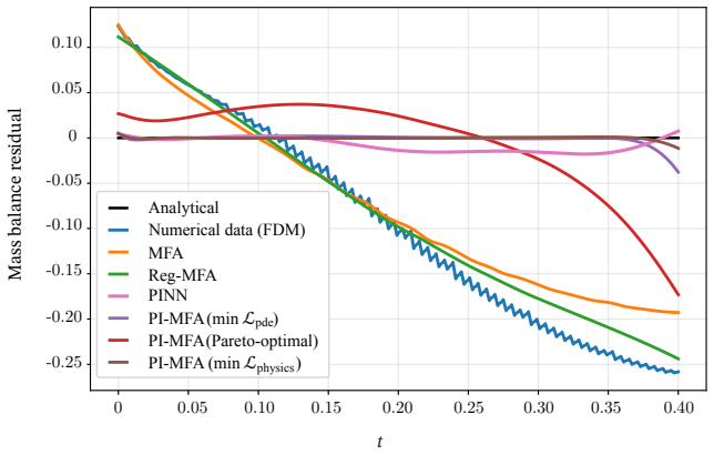
- Reconstructed fields exhibit reduced PDE residuals and better global balance-law consistency.
- Lower approximation errors occur when the input data is physically inconsistent.
- The method offers computational advantages over physics-informed neural networks for the tested equations.
- Continuous fields remain compact and locally supported, enabling efficient downstream analysis and visualization.
Where Pith is reading between the lines
- Such reconstructions could improve reliability of derived quantities like gradients or integrals computed from discrete simulation outputs.
- The framework might apply to other types of physical data beyond fluid flows if the governing equations are known.
- Integration with existing simulation codes could allow on-the-fly physics-informed post-processing without full field storage.
Load-bearing premise
The optimization balancing data fidelity with PDE residuals can be solved to produce B-spline coefficients that meaningfully reduce physical residuals in the tested problems.
What would settle it
Numerical experiments on the listed flow equations where the PI-MFA fields do not show lower PDE residuals or improved balance consistency relative to standard MFA.
Figures


read the original abstract
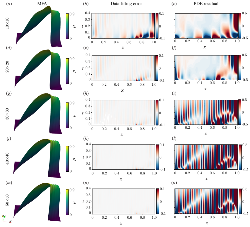
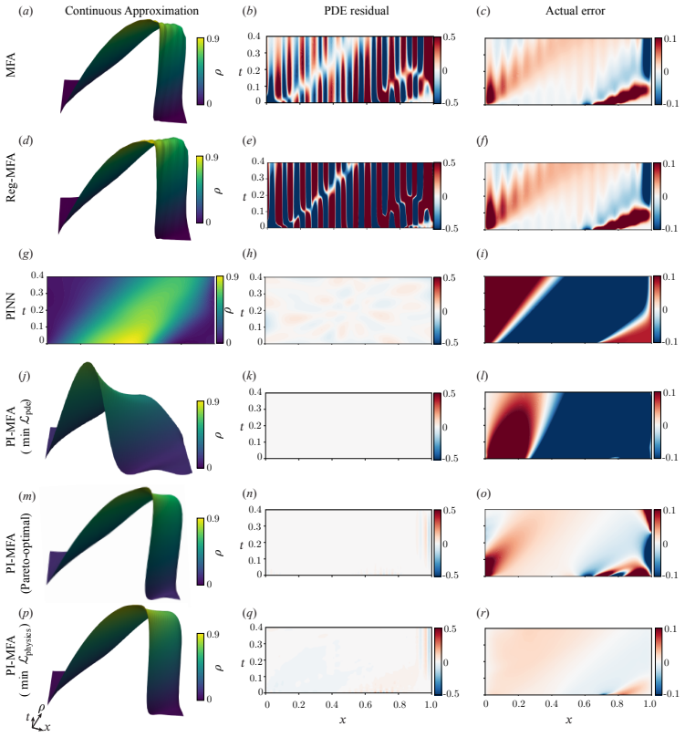
Continuous approximations of flow data are useful for downstream analysis, differentiation, and visualization, but purely data-driven reconstructions do not, in general, preserve the governing physics. This limitation becomes particularly important when input data are physically inconsistent, whether due to low-fidelity discretizations or unmodeled discrepancies. In such cases, reconstructed fields may exhibit inaccurate PDE residuals, violated balance laws, or unreliable derived quantities. To address this, we propose a physics-informed B-spline framework that embeds physical constraints directly into the reconstruction process. The method constructs compact, continuously differentiable representations of discrete fields using tensor-product B-splines and determines spline control points by solving an optimization problem balancing data fidelity with residuals of the governing PDEs, alongside initial and boundary conditions. Leveraging exact analytical derivatives of the B-spline basis enables efficient and accurate evaluation of physical residuals without storing full-resolution fields. We refer to this approach as physics-informed multivariate functional approximation (PI-MFA). Numerical studies on the 1D convection-diffusion, 2D coupled Burgers, and 2D incompressible Navier-Stokes equations show PI-MFA reduces PDE residuals and improves global balance-law consistency. Compared with standard and regularized MFA, PI-MFA produces more physically faithful reconstructions and, for physically inconsistent data, lower approximation errors, while offering computational advantages over tested physics-informed neural networks. Overall, PI-MFA preserves the compactness, local support, and exact differentiability of classical spline spaces while producing reliable continuous flow fields for scientific analysis and visualization.
Editorial analysis
A structured set of objections, weighed in public.
Referee Report
Summary. The manuscript introduces physics-informed multivariate functional approximation (PI-MFA), a framework that represents discrete flow data via tensor-product B-splines and determines the control points through an optimization that balances data-fidelity terms against PDE residuals together with initial and boundary conditions. Exact analytic derivatives of the B-spline basis are used to evaluate the physics residuals efficiently. Numerical demonstrations are reported on the 1D convection-diffusion equation, the 2D coupled Burgers equations, and the 2D incompressible Navier-Stokes equations, with the claim that PI-MFA yields lower PDE residuals, improved global balance-law consistency, and smaller approximation errors on physically inconsistent data than standard or regularized MFA while remaining computationally cheaper than the tested physics-informed neural networks.
Significance. If the reported improvements are quantitatively confirmed, the method supplies a compact, locally supported, and exactly differentiable alternative to neural-network-based physics-informed reconstructions. The use of analytic B-spline derivatives for residual evaluation without storing full-resolution fields is a clear technical advantage for downstream analysis and visualization tasks.
major comments (1)
- [Abstract / Numerical studies] Abstract and Numerical studies section: the central claim that 'numerical studies ... show PI-MFA reduces PDE residuals and improves global balance-law consistency' and produces 'lower approximation errors' is not accompanied by any quantitative metrics, error norms, residual values, error bars, optimization tolerances, or data-exclusion criteria. Without these numbers the support for the load-bearing assertion that the physics-informed optimization yields meaningfully better reconstructions cannot be assessed.
minor comments (1)
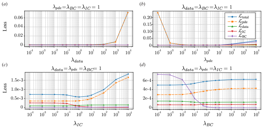
- The balancing weights between the data and physics terms are free parameters; a brief sensitivity study or default selection strategy would clarify reproducibility.
Simulated Author's Rebuttal
We thank the referee for their thorough review and constructive feedback on our manuscript. We address the major comment below and will revise the manuscript to incorporate the suggested quantitative details.
read point-by-point responses
-
Referee: [Abstract / Numerical studies] Abstract and Numerical studies section: the central claim that 'numerical studies ... show PI-MFA reduces PDE residuals and improves global balance-law consistency' and produces 'lower approximation errors' is not accompanied by any quantitative metrics, error norms, residual values, error bars, optimization tolerances, or data-exclusion criteria. Without these numbers the support for the load-bearing assertion that the physics-informed optimization yields meaningfully better reconstructions cannot be assessed.
Authors: We agree that explicit quantitative metrics are needed to substantiate the claims regarding reduced PDE residuals, improved balance-law consistency, and lower approximation errors. In the revised version, we will augment the Numerical studies section with tables reporting L2 and L-infinity norms of PDE residuals, global mass/momentum balance errors, and data approximation errors for PI-MFA versus standard MFA, regularized MFA, and the tested PINNs on each benchmark problem. We will also document the optimization tolerances employed (e.g., convergence criteria for the control-point solver) and any data-exclusion criteria used in the experiments. These additions will allow direct quantitative assessment of the improvements. revision: yes
Circularity Check
No significant circularity; method is an explicit optimization construction
full rationale
The paper defines PI-MFA as the solution of an optimization problem whose objective explicitly combines a data-fidelity term with PDE-residual, initial-condition, and boundary-condition terms; the B-spline representation and its analytic derivatives are standard and independent of the target flow fields. Numerical studies are empirical demonstrations on standard test problems rather than predictions that reduce to the fitted inputs by construction. No self-citation is invoked as a load-bearing uniqueness theorem, no ansatz is smuggled via prior work, and no renaming of known results occurs. The derivation chain is therefore self-contained against external benchmarks.
Axiom & Free-Parameter Ledger
free parameters (1)
- balancing weights between data and physics terms
axioms (1)
- domain assumption Tensor-product B-splines possess sufficient approximation power to represent the solution fields of the tested PDEs while allowing exact derivative evaluation
Reference graph
Works this paper leans on
-
[1]
L. Piegl, W. Tiller, The NURBS Book, 2nd Edition, Springer, Berlin, Heidelberg, 1997.doi: 10.1007/978-3-642-59223-2
-
[2]
de Boor, A Practical Guide to Splines, revised Edition, Vol
C. de Boor, A Practical Guide to Splines, revised Edition, Vol. 27 of Applied Mathematical Sciences, Springer, New York, 2001.doi:10.1007/978-1-4612-6333-3
-
[3]
L. L. Schumaker, Spline Functions: Basic Theory, 3rd Edition, Cambridge Mathematical Library, Cambridge University Press, Cambridge, 2007.doi:10.1017/CBO9780511618994
-
[4]
P. H. C. Eilers, B. D. Marx, Flexible smoothing with B-splines and penalties, Statistical Science 11 (2) (1996) 89–121.doi:10.1214/ss/1038425655
-
[5]
M. J. Johnson, Z. Shen, Y. Xu, Scattered data reconstruction by regularization in B-spline and associated wavelet spaces, Journal of Approximation Theory 159 (2) (2009) 197–223.doi:10.1016/j.jat. 2009.02.005
-
[6]
S. Merchel, B. J¨ uttler, D. Mokriˇs, M. Pan, Fast formation of matrices for least-squares fitting by tensor- product spline surfaces, Computer-Aided Design 150 (2022) 103307.doi:10.1016/j.cad.2022. 103307
-
[7]
T. J. R. Hughes, J. A. Cottrell, Y. Bazilevs, Isogeometric analysis: CAD, finite elements, NURBS, exact geometry and mesh refinement, Computer Methods in Applied Mechanics and Engineering 194 (39–41) (2005) 4135–4195.doi:10.1016/j.cma.2004.10.008
-
[8]
Y. Bazilevs, L. Beir ˜ao da Veiga, J. A. Cottrell, T. J. R. Hughes, G. Sangalli, Isogeometric analysis: approximation, stability and error estimates forℎ-refined meshes, Mathematical Models and Methods in Applied Sciences 16 (7) (2006) 1031–1090.doi:10.1142/S0218202506001455
-
[9]
J. A. Cottrell, T. J. R. Hughes, A. Reali, Studies of refinement and continuity in isogeometric structural analysis, Computer Methods in Applied Mechanics and Engineering 196 (41–44) (2007) 4160–4183. doi:10.1016/j.cma.2007.04.007
-
[10]
F. Auricchio, L. Beir ˜ao da Veiga, T. J. R. Hughes, A. Reali, G. Sangalli, Isogeometric collocation methods, Mathematical Models and Methods in Applied Sciences 20 (11) (2010) 2075–2107.doi: 10.1142/S0218202510004878
-
[11]
F. Auricchio, L. Beir ˜ao da Veiga, T. J. R. Hughes, A. Reali, G. Sangalli, Isogeometric collocation for elastostatics and explicit dynamics, Computer Methods in Applied Mechanics and Engineering 249–252 (2012) 2–14.doi:10.1016/j.cma.2012.03.026
-
[13]
M. Montardini, G. Sangalli, L. Tamellini, Optimal-order isogeometric collocation at Galerkin super- convergent points, Computer Methods in Applied Mechanics and Engineering 316 (2017) 741–757. doi:10.1016/j.cma.2016.09.043
-
[14]
T. Peterka, Y. S. G. Nashed, I. R. Grindeanu, V. S. Mahadevan, R. Yeh, X. Tricoche, Foundations of multivariate functional approximation for scientific data, in: 2018 IEEE 8th Symposium on Large Data Analysis and Visualization (LDA V), 2018, pp. 61–71.doi:10.1109/LDAV.2018.8739195. 55
-
[15]
D. Lenz, R. Yeh, V. Mahadevan, I. Grindeanu, T. Peterka, Customizable adaptive regularization techniques for B-spline modeling, Journal of Computational Science 71 (2023) 102037.doi:10. 1016/j.jocs.2023.102037
arXiv 2023
-
[16]
J. Sun, D. Lenz, H. Yu, T. Peterka, Scalable volume visualization for big scientific data modeled by functional approximation, IEEE Transactions on Visualization and Computer Graphics 30 (12) (2024) 8637–8651.doi:10.1109/TVCG.2024.3353594
-
[17]
J. Sun, D. Lenz, H. Yu, T. Peterka, MFA-DVR: Direct volume rendering of MFA models, Journal of Visualization 27 (2024) 109–126.doi:10.1007/s12650-023-00946-y
-
[18]
T. Peterka, D. Lenz, I. Grindeanu, V. S. Mahadevan, Towards adaptive refinement for multivariate functional approximation of scientific data, in: 2023 IEEE 13th Symposium on Large Data Analysis and Visualization (LDA V), 2023, pp. 32–41.doi:10.1109/LDAV60332.2023.00011
-
[19]
I. Grindeanu, T. Peterka, V. S. Mahadevan, Y. S. G. Nashed, Scalable, high-order continuity across block boundaries of functional approximations computed in parallel, in: 2019 IEEE International Conference on Cluster Computing (CLUSTER), 2019, pp. 1–9.doi:10.1109/CLUSTER.2019.8891018
-
[20]
V. S. Mahadevan, D. Lenz, I. Grindeanu, T. Peterka, Accelerating multivariate functional approximation computation with domain decomposition techniques, Journal of Computational Science 78 (2024) 102268.doi:10.1016/j.jocs.2024.102268
-
[21]
G. Ma, D. Lenz, T. Peterka, H. Guo, B. Wang, Critical point extraction from multivariate functional approximation, in: 2024 IEEE Topological Data Analysis and Visualization (TopoInVis), 2024, pp. 12–22.doi:10.1109/TopoInVis64104.2024.00006
-
[22]
J. Sun, D. Lenz, H. Yu, T. Peterka, Adaptive multi-resolution encoding for interactive large-scale volume visualization through functional approximation, in: 2024 IEEE 14th Symposium on Large Data Analysis and Visualization (LDA V), IEEE, 2024, pp. 33–42.doi:10.1109/LDAV64567.2024.00006
-
[23]
M. Guo, A. Manzoni, M. Amendt, P. Conti, J. S. Hesthaven, Multi-fidelity regression using artificial neural networks: Efficient approximation of parameter-dependent output quantities, Computer Methods in Applied Mechanics and Engineering 389 (2022) 114378.doi:10.1016/j.cma.2021.114378
-
[24]
A. A. Howard, M. Perego, G. E. Karniadakis, P. Stinis, Multifidelity deep operator networks for data-driven and physics-informed problems, Journal of Computational Physics 493 (2023) 112462. doi:10.1016/j.jcp.2023.112462
-
[25]
A. Kiener, S. Langer, P. Bekemeyer, Data-driven correction of coarse grid CFD simulations, Computers & Fluids 264 (2023) 105971.doi:10.1016/j.compfluid.2023.105971
-
[26]
S. Kang, E. M. Constantinescu, Learning subgrid-scale models with neural ordinary differential equa- tions, Computers & Fluids 261 (2023) 105919.doi:10.1016/j.compfluid.2023.105919
-
[27]
P. Sousa, C. V. Rodrigues, A. Afonso, Enhancing CFD solver with machine learning techniques, Computer Methods in Applied Mechanics and Engineering 429 (2024) 117133.doi:10.1016/j. cma.2024.117133
work page doi:10.1016/j 2024
-
[28]
S. Kang, E. M. Constantinescu, Enhancing low-order discontinuous Galerkin methods with neural ordinary differential equations for compressible Navier–Stokes equations (2025).arXiv:2310.18897, doi:10.48550/arXiv.2310.18897
-
[29]
J. Jung, E. Constantinescu, Learning differentiable weak-form corrections to accelerate finite element simulations (2026).arXiv:2601.20019,doi:10.48550/arXiv.2601.20019
-
[30]
S. Garg, S. Chakraborty, B. Hazra, Physics-integrated hybrid framework for model form error identifi- cation in nonlinear dynamical systems, Mechanical Systems and Signal Processing 173 (2022) 109039. doi:10.1016/j.ymssp.2022.109039. 56
-
[31]
M. Raissi, P. Perdikaris, G. E. Karniadakis, Physics-informed neural networks: A deep learning framework for solving forward and inverse problems involving nonlinear partial differential equations, Journal of Computational Physics 378 (2019) 686–707.doi:10.1016/j.jcp.2018.10.045
-
[32]
J. Yu, L. Lu, X. Meng, G. E. Karniadakis, Gradient-enhanced physics-informed neural networks for forward and inverse PDE problems, Computer Methods in Applied Mechanics and Engineering 393 (2022) 114823.doi:10.1016/j.cma.2022.114823
-
[33]
D. Shu, Z. Li, A. Barati Farimani, A physics-informed diffusion model for high-fidelity flow field reconstruction, Journal of Computational Physics 478 (2023) 111972.doi:10.1016/j.jcp.2023. 111972
-
[34]
B. L¨ utjens, B. Leshchinskiy, C. Requena-Mesa, F. Chishtie, N. D´ıaz-Rodr´ıguez, O. Boulais, A. Pi˜na, D. Newman, A. Lavin, Y. Gal, C. Ra¨ıssi, Physics-informed GANs for coastal flood visualization (2020). arXiv:2010.08103,doi:10.48550/arXiv.2010.08103
-
[35]
A. Chakravarty, S. Misra, C. S. Rai, Visualization of hydraulic fracture using physics-informed cluster- ing to process ultrasonic shear waves, International Journal of Rock Mechanics and Mining Sciences 137 (2021) 104568.doi:10.1016/j.ijrmms.2020.104568
-
[36]
C. Banerjee, K. Nguyen, C. Fookes, G. E. Karniadakis, Physics-informed computer vision: A review and perspectives, ACM Computing Surveys 57 (1) (2024) 1–38.doi:10.1145/3689037
-
[37]
N. Ohashi, L. K. Hwang, B. Kwon, Physics-informed neural networks for multi-field visualization with single-color laser induced fluorescence, AI Thermal Fluids 1 (2025) 100005.doi:10.1016/j.aitf. 2025.100005
-
[38]
M. G. Cox, The numerical evaluation of B-splines, IMA Journal of Applied Mathematics 10 (2) (1972) 134–149.doi:10.1093/imamat/10.2.134
-
[39]
de Boor, On calculating with B-splines, Journal of Approximation Theory 6 (1) (1972) 50–62
C. de Boor, On calculating with B-splines, Journal of Approximation Theory 6 (1) (1972) 50–62. doi:10.1016/0021-9045(72)90080-9
-
[40]
D. C. Liu, J. Nocedal, On the limited memory BFGS method for large scale optimization, Mathematical Programming 45 (1–3) (1989) 503–528.doi:10.1007/BF01589116
-
[41]
Qiu, LBFGS++ (LBFGSpp): A header-only C++ library for L-BFGS and L-BFGS-B algorithms, GitHub repository, version v0.4.0, commit c524a40 (2025)
Y. Qiu, LBFGS++ (LBFGSpp): A header-only C++ library for L-BFGS and L-BFGS-B algorithms, GitHub repository, version v0.4.0, commit c524a40 (2025). URLhttps://github.com/yixuan/LBFGSpp
2025
-
[42]
Crank, The Mathematics of Diffusion, 2nd Edition, Clarendon Press, Oxford, 1975
J. Crank, The Mathematics of Diffusion, 2nd Edition, Clarendon Press, Oxford, 1975
1975
-
[43]
Haberman, Applied Partial Differential Equations: With Fourier Series and Boundary Value Prob- lems, 5th Edition, Pearson, Boston, 2013
R. Haberman, Applied Partial Differential Equations: With Fourier Series and Boundary Value Prob- lems, 5th Edition, Pearson, Boston, 2013
2013
-
[44]
D. Lenz, O. Marin, V. S. Mahadevan, R. Yeh, T. Peterka, Fourier-informed knot placement schemes for B-spline approximation, Mathematics and Computers in Simulation 213 (2023) 374–393.doi: 10.1016/j.matcom.2023.05.017
-
[45]
Pareto, Manual of Political Economy, A
V. Pareto, Manual of Political Economy, A. M. Kelley, New York, 1971
1971
-
[46]
R. T. Marler, J. S. Arora, Survey of multi-objective optimization methods for engineering, Structural and Multidisciplinary Optimization 26 (6) (2004) 369–395.doi:10.1007/s00158-003-0368-6
-
[47]
R. T. Marler, J. S. Arora, The weighted sum method for multi-objective optimization: new in- sights, Structural and Multidisciplinary Optimization 41 (6) (2010) 853–862.doi:10.1007/ s00158-009-0460-7
2010
-
[48]
F. M. Rohrhofer, S. Posch, C. G ¨oßnitzer, B. C. Geiger, Data vs. physics: The apparent Pareto front of physics-informed neural networks, IEEE Access 11 (2023) 86252–86261.arXiv:2105.00862, doi:10.1109/ACCESS.2023.3302892. 57
-
[49]
F. Heldmann, S. Berkhahn, M. Ehrhardt, K. Klamroth, PINN training using biobjective optimization: The trade-off between data loss and residual loss, Journal of Computational Physics 488 (2023) 112211. doi:10.1016/j.jcp.2023.112211
-
[50]
R. Bischof, M. A. Kraus, Multi-objective loss balancing for physics-informed deep learning, Computer Methods in Applied Mechanics and Engineering 439 (2025) 117914.doi:10.1016/j.cma.2025. 117914
-
[51]
J. D. Cole, On a quasi-linear parabolic equation occurring in aerodynamics, Quarterly of Applied Mathematics 9 (3) (1951) 225–236.doi:10.1090/qam/42889
-
[52]
R. J. LeVeque, Finite Volume Methods for Hyperbolic Problems, Cambridge University Press, Cam- bridge, 2002.doi:10.1017/CBO9780511791253
-
[53]
P. Clark di Leoni, A. N. Hirata, P. D. Mininni, Dynamics of partially thermalized solutions of the Burgers equation, Physical Review Fluids 3 (2018) 014603.doi:10.1103/PhysRevFluids.3.014603
-
[54]
L. C. Evans, Partial Differential Equations, 2nd Edition, Vol. 19 of Graduate Studies in Mathematics, American Mathematical Society, Providence, RI, 2010
2010
-
[55]
Borthwick, Introduction to Partial Differential Equations, Springer, Cham, 2017.doi:10.1007/ 978-3-319-48936-0
D. Borthwick, Introduction to Partial Differential Equations, Springer, Cham, 2017.doi:10.1007/ 978-3-319-48936-0
2017
-
[56]
M. C. Kennedy, A. O’Hagan, Bayesian calibration of computer models, Journal of the Royal Statistical Society: Series B (Statistical Methodology) 63 (3) (2001) 425–464.doi:10.1111/1467-9868. 00294
-
[57]
Hooker, Forcing function diagnostics for nonlinear dynamics, Biometrics 65 (3) (2009) 928–936
G. Hooker, Forcing function diagnostics for nonlinear dynamics, Biometrics 65 (3) (2009) 928–936. doi:10.1111/j.1541-0420.2008.01172.x
-
[58]
R. E. Morrison, T. A. Oliver, R. D. Moser, Representing model inadequacy: A stochastic operator approach, SIAM/ASA Journal on Uncertainty Quantification 6 (2) (2018) 457–496.doi:10.1137/ 16M1106419
2018
-
[59]
A. Masud, S. Nashar, S. A. Goraya, Physics-constrained data-driven variational method for missing physics and model-form error, Computer Methods in Applied Mechanics and Engineering 417 (2023) 116295.doi:10.1016/j.cma.2023.116295
-
[60]
D. A. Ham, P. H. J. Kelly, L. Mitchell, C. J. Cotter, R. C. Kirby, K. Sagiyama, N. Bouziani, S. Vorder- wuelbecke, T. J. Gregory, J. Betteridge, D. R. Shapero, R. W. Nixon-Hill, C. J. Ward, P. E. Farrell, P. D. Brubeck, I. Marsden, T. H. Gibson, M. Homolya, T. Sun, A. T. T. McRae, F. Luporini, A. Gregory, M. Lange, S. W. Funke, F. Rathgeber, G.-T. Bercea,...
-
[61]
U. Ghia, K. N. Ghia, C. T. Shin, High-Re solutions for incompressible flow using the Navier–Stokes equations and a multigrid method, Journal of Computational Physics 48 (3) (1982) 387–411.doi: 10.1016/0021-9991(82)90058-4
-
[62]
J. Shen, Hopf bifurcation of the unsteady regularized driven cavity flow, Journal of Computational Physics 95 (1) (1991) 228–245.doi:10.1016/0021-9991(91)90261-I
-
[63]
D. Kochkov, J. A. Smith, A. Alieva, Q. Wang, M. P. Brenner, S. Hoyer, Machine learning-accelerated computational fluid dynamics, Proceedings of the National Academy of Sciences 118 (21) (2021) e2101784118.doi:10.1073/pnas.2101784118
-
[64]
J. Pathak, M. Mustafa, K. Kashinath, E. Motheau, T. Kurth, M. Day, Using machine learning to augment coarse-grid computational fluid dynamics simulations (2020).arXiv:2010.00072,doi: 10.48550/arXiv.2010.00072. 58
-
[65]
Z. Li, N. Kovachki, K. Azizzadenesheli, B. Liu, K. Bhattacharya, A. Stuart, A. Anandkumar, Fourier neural operator for parametric partial differential equations, in: International Conference on Learning Representations, 2021.arXiv:2010.08895,doi:10.48550/arXiv.2010.08895. URLhttps://openreview.net/forum?id=c8P9NQVtmnO
work page internal anchor Pith review Pith/arXiv arXiv doi:10.48550/arxiv.2010.08895 2021
-
[66]
T. J. R. Hughes, The Finite Element Method: Linear Static and Dynamic Finite Element Analysis, Prentice-Hall, Englewood Cliffs, NJ, 1987
1987
-
[67]
A. Ern, J.-L. Guermond, Theory and Practice of Finite Elements, Vol. 159 of Applied Mathematical Sciences, Springer, New York, 2004.doi:10.1007/978-1-4757-4355-5
-
[68]
M. Raissi, A. Yazdani, G. E. Karniadakis, Hidden fluid mechanics: Learning velocity and pressure fields from flow visualizations, Science 367 (6481) (2020) 1026–1030.doi:10.1126/science.aaw4741
-
[69]
J. A. Cottrell, T. J. R. Hughes, Y. Bazilevs, Isogeometric Analysis: Toward Integration of CAD and FEA, Wiley, Chichester, 2009.doi:10.1002/9780470749081. Government License (will be removed at publication): The submitted manuscript has been created by UChicago Argonne, LLC, Operator of Argonne National Laboratory (“Argonne”). Argonne, a U.S. Department o...
discussion (0)
Sign in with ORCID, Apple, or X to comment. Anyone can read and Pith papers without signing in.