VEQ: a fast parametric Grad--Shafranov solver for fixed-boundary tokamak equilibria with flexible source profiles
Pith reviewed 2026-06-27 08:16 UTC · model grok-4.3
The pith
VEQ computes fixed-boundary tokamak equilibria in milliseconds via a parametric MXH-Chebyshev representation.
A machine-rendered reading of the paper's core claim, the machinery that carries it, and where it could break.
Core claim
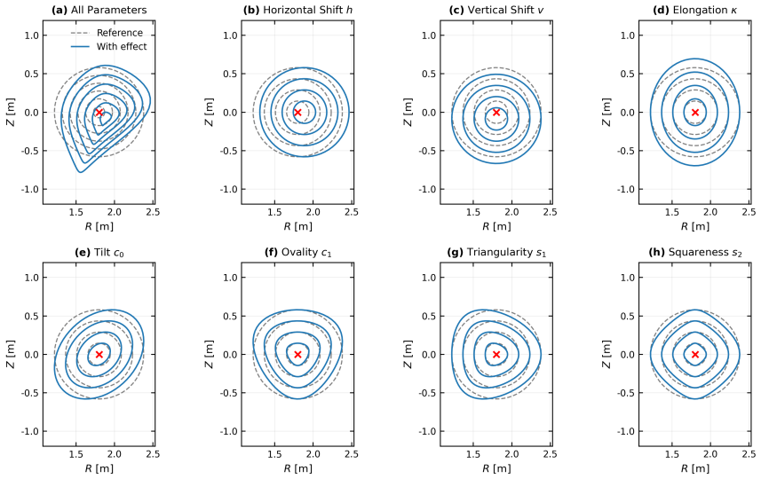
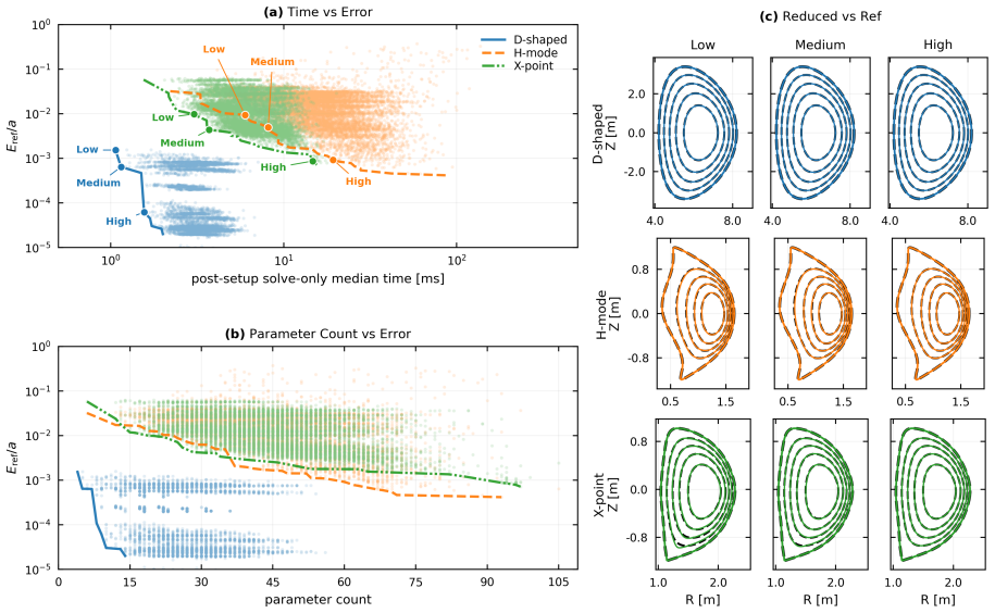
VEQ enforces a variationally induced projected residual on MXH-type flux-surface harmonics and shifted-Chebyshev coefficients for radial profiles and source closures, allowing consistent fixed-boundary solutions from six different input routes with shape errors below 2e-3 and solve times under 20 ms for selected reduced configurations.
What carries the argument
Finite-dimensional MXH-type flux-surface harmonics combined with shifted-Chebyshev coefficients, closed under a variationally induced projected residual operator that accepts six route-specific input closures.
If this is right
- All six input routes map to the identical residual operator, producing consistent equilibria for mutually compatible smooth inputs.
- Reduced representations achieve minor-radius-normalized shape errors between 1.1e-3 and 1.9e-3 with solve-only median times from 1.6 ms to 19 ms.
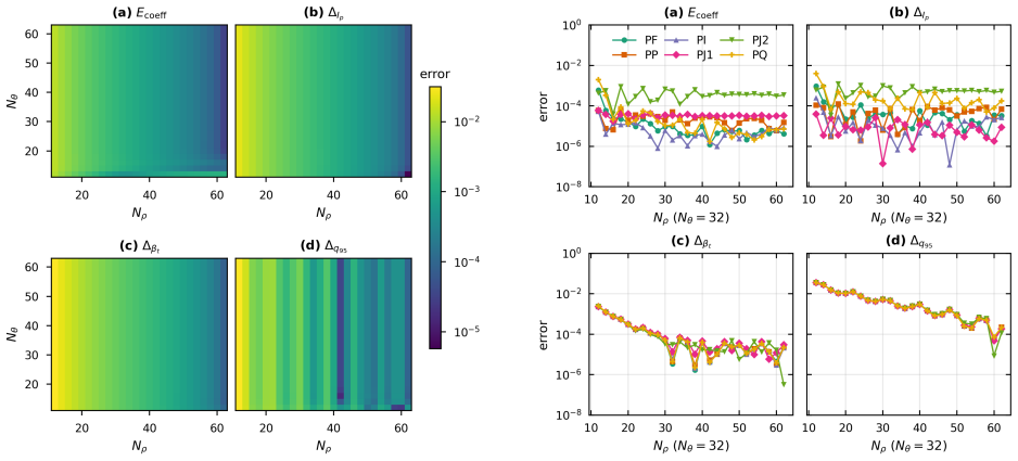
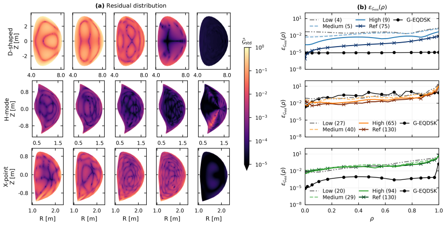
- Enriching the active parameter count improves interior force balance while global error metrics stay dominated by boundary contributions.
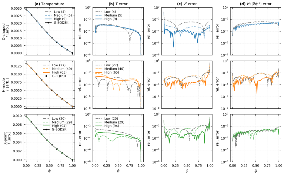
- One-dimensional transport-geometry coupling against G-EQDSK target geometry yields temperature-profile responses below one percent.
Where Pith is reading between the lines
- The approach could support workflows that query equilibria thousands of times by keeping most solves at reduced fidelity and reserving full solves for flagged cases.
- Automated pointwise residual checks could be inserted into iterative loops to decide when boundary refinement or higher-order representations are required.
- The same harmonic-plus-polynomial closure might be tested on time-dependent or mildly non-axisymmetric cases to check whether the low-latency property survives.
Load-bearing premise
The finite-dimensional MXH-plus-Chebyshev representation with selected parameter counts produces equilibria whose interior force balance is adequate for target workflows even when global RMS errors remain dominated by near-boundary contributions.
What would settle it
Direct inspection of pointwise strong-form Grad-Shafranov residuals across the interior versus near-boundary regions for the H-mode and X-point test cases would show whether interior balance meets workflow requirements.
Figures
read the original abstract
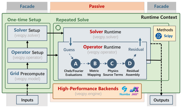
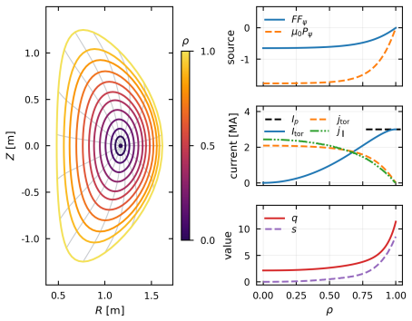
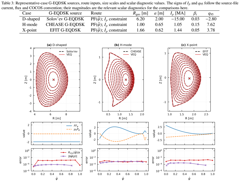
Veloce EQuilibrium (VEQ) is a compact parametric framework for tokamak modeling workflows that repeatedly query continuous fixed-boundary equilibria at low latency. The VEQPy implementation evaluated here is an axisymmetric fixed-boundary Grad-Shafranov solver whose main solve enforces a variationally induced projected residual. Its active unknowns are MXH-type flux-surface harmonics and shifted-Chebyshev coefficients for radial profile and source closures. Six input routes accept pressure-gradient, toroidal-field-function, poloidal-flux-gradient, enclosed toroidal current, current-density and safety-factor information through route-specific closures, while all routes map to the same finite-dimensional residual operator. Controlled tests show route consistency for smooth, mutually compatible inputs generated from a common reference equilibrium. For Pareto-selected reduced configurations in three G-EQDSK cases, the most accurate selected rows correspond to a D-shaped case (9 active parameters, minor-radius-normalized shape error 1.4e-3, solve-only median 1.6 ms), an H-mode case (65, 1.1e-3, 19 ms), and an X-point case treated as a smoothed fixed-boundary representation of a diverted boundary (94, 1.9e-3, 15 ms). Sampled pointwise strong-form Grad-Shafranov diagnostics show that enriching the active representation mainly improves interior force balance, whereas the global RMS and maximum values for the H-mode and X-point cases remain dominated by near-boundary contributions. In an isolated one-dimensional transport-geometry coupling test against the target geometry read from G-EQDSK, the temperature-profile response remains below about one percent. These results support using VEQ for repeated equilibrium-geometry queries, provided that pointwise diagnostics are retained to screen cases requiring boundary refinement, local correction or higher-fidelity equilibrium solves.
Editorial analysis
A structured set of objections, weighed in public.
Referee Report
Summary. The paper introduces VEQ, a compact parametric Grad-Shafranov solver for fixed-boundary tokamak equilibria that enforces a variationally induced projected residual over a finite-dimensional space of MXH-type flux-surface harmonics and shifted-Chebyshev coefficients. It supports six input routes that map to the same residual operator, reports route-consistency tests on compatible inputs, and gives Pareto-selected performance (solve time, shape error) on three G-EQDSK cases together with pointwise strong-form diagnostics and one 1-D transport-geometry coupling test.
Significance. If the interior force-balance residuals remain small enough after Pareto selection, the method could support low-latency repeated equilibrium queries in modeling workflows while retaining pointwise screening; the route-consistency tests and explicit performance numbers on G-EQDSK cases are concrete strengths that would be retained under revision.
major comments (3)
- [Abstract] Abstract (performance paragraph on G-EQDSK cases): the claim that enriching the MXH+Chebyshev representation improves interior force balance is not accompanied by quantitative bounds on the retained interior residuals; because global RMS/max errors remain near-boundary dominated for the H-mode and X-point cases, it is unclear whether the 2-D interior residuals are small enough for downstream transport/geometry queries. The single 1-D coupling test does not address 2-D propagation of boundary-layer errors.
- [Abstract] Abstract: the Pareto-selected active-parameter counts (9/65/94) are chosen after the fact on the three test cases; without an a-priori criterion or sensitivity study showing that these finite-dimensional spaces generically produce adequate interior equilibria, the central numerical claim that the representation is sufficient for the target workflows rests on post-hoc selection.
- [Abstract] Abstract: the variationally induced projected residual and the explicit residual operator are invoked as the main solve but are not derived or written out; without these the route-consistency tests and pointwise diagnostics cannot be independently verified.
minor comments (2)
- [Abstract] The abstract states that pointwise diagnostics should be retained to screen cases, but does not specify the diagnostic thresholds or how they would be implemented in the VEQPy code.
- [Abstract] Notation for the six input routes and the mapping to the common residual operator is introduced without an accompanying table or diagram that would clarify the closures for each route.
Simulated Author's Rebuttal
We thank the referee for the constructive comments on our manuscript. We respond point-by-point to the three major comments below, indicating where revisions will be made.
read point-by-point responses
-
Referee: [Abstract] Abstract (performance paragraph on G-EQDSK cases): the claim that enriching the MXH+Chebyshev representation improves interior force balance is not accompanied by quantitative bounds on the retained interior residuals; because global RMS/max errors remain near-boundary dominated for the H-mode and X-point cases, it is unclear whether the 2-D interior residuals are small enough for downstream transport/geometry queries. The single 1-D coupling test does not address 2-D propagation of boundary-layer errors.
Authors: We agree that explicit quantitative bounds on interior residuals would strengthen the presentation. In the revised manuscript we will add L2-norm interior residuals (computed after excluding a thin boundary layer) for the three Pareto-selected cases, directly supporting the statement that enrichment improves interior force balance. We also acknowledge that the single 1-D coupling test does not address 2-D error propagation and will add an explicit caveat in the abstract and discussion recommending retention of pointwise diagnostics for workflows sensitive to boundary-layer errors. revision: yes
-
Referee: [Abstract] Abstract: the Pareto-selected active-parameter counts (9/65/94) are chosen after the fact on the three test cases; without an a-priori criterion or sensitivity study showing that these finite-dimensional spaces generically produce adequate interior equilibria, the central numerical claim that the representation is sufficient for the target workflows rests on post-hoc selection.
Authors: The reported counts are obtained by Pareto selection on the three specific G-EQDSK cases to illustrate the performance achievable with the MXH+Chebyshev basis. The manuscript does not assert a universal a-priori rule for dimension selection; it presents the results as concrete, case-specific evidence that the representation can reach the quoted shape errors while mapping all six routes to the same residual operator. We will expand the methods section to describe the Pareto procedure more explicitly and add a short discussion of how the selected dimensions relate to the observed interior residual improvement, but a comprehensive sensitivity study over a wider ensemble is outside the scope of the present work. revision: partial
-
Referee: [Abstract] Abstract: the variationally induced projected residual and the explicit residual operator are invoked as the main solve but are not derived or written out; without these the route-consistency tests and pointwise diagnostics cannot be independently verified.
Authors: The derivation of the variationally induced projected residual, the finite-dimensional MXH+Chebyshev space, and the explicit residual operator (including the route-specific closures that all map to the same operator) appears in Section 3 of the full manuscript, with the mathematical statements given in Equations (3)–(7). The route-consistency tests and pointwise diagnostics are performed with respect to that operator. We will add a forward reference to Section 3 already in the abstract and will ensure the key equations are reproduced or clearly cited in any revised abstract to improve accessibility. revision: yes
Circularity Check
No significant circularity detected
full rationale
The paper describes a standard numerical discretization of the fixed-boundary Grad-Shafranov equation via a variationally projected residual on a finite-dimensional MXH-plus-Chebyshev space. Input routes map to the same residual operator, and reported diagnostics (shape errors, solve times, pointwise residuals) are direct outputs of that discretization applied to reference G-EQDSK data. No equation reduces a claimed prediction or result to a fitted quantity defined from the same data, no self-citation is load-bearing for the central claims, and no uniqueness theorem or ansatz is imported from prior author work. The derivation chain is therefore self-contained against external benchmarks.
Axiom & Free-Parameter Ledger
free parameters (1)
- Number of active MXH harmonics and shifted-Chebyshev coefficients
axioms (2)
- domain assumption Axisymmetric fixed-boundary tokamak equilibrium obeys the Grad-Shafranov equation
- domain assumption Variational projected residual minimization yields a valid discrete solution to the Grad-Shafranov equation
Reference graph
Works this paper leans on
-
[1]
F. Imbeaux, S. D. Pinches, J. B. Lister, et al., Design and first applications of the ITER integrated modelling & analysis suite, Nuclear Fusion 55 (2015) 123006. doi:10.1088/0029-5515/55/12/123006
-
[2]
F. Felici, J. Citrin, A. Teplukhina, J. Redondo, C. Bourdelle, F. Imbeaux, O. Sauter, et al., Real-time-capable prediction of temperature and density profiles in a tokamak using RAPTOR and a first-principle-based transport model, Nuclear Fusion 58 (2018) 096006. doi:10.1088/1741-4326/aac8f0
-
[3]
S. W. Haney, W. L. Barr, J. A. Crotinger, L. J. Perkins, C. J. Solomon, E. A. Chaniotakis, J. P. Freidberg, J. Wei, J. D. Galambos, J. Mandrekas, A “supercode” for systems analysis of tokamak experiments and reactors, Fusion Technology 21 (1992) 1749–1758. doi:10.13182/fst92-a29974
-
[4]
V . D. Shafranov, Plasma equilibrium in a magnetic field, Reviews of Plasma Physics 2 (1966) 103. Edited by M. A. Leontovich; Consultants Bureau, New York
1966
-
[5]
H. Grad, H. Rubin, Hydromagnetic equilibria and force-free fields, in: Proceedings of the Second United Nations International Conference on the Peaceful Uses of Atomic Energy, volume 31, Geneva, 1958, p. 190
1958
-
[6]
M. D. Kruskal, R. M. Kulsrud, Equilibrium of a magnetically confined plasma in a toroid, The Physics of Fluids 1 (1958) 265–274. doi:10.1063/1.1705884
-
[7]
J. M. Greene, J. L. Johnson, K. E. Weimer, Tokamak equilibrium, The Physics of Fluids 14 (1971) 671–683. doi:10.1063/1.1693488
-
[8]
L. Lao, H. St. John, R. Stambaugh, A. Kellman, W. Pfeiffer, Reconstruction of current profile parameters and plasma shapes in tokamaks, Nuclear Fusion 25 (1985) 1611–1622. doi:10.1088/0029-5515/25/11/007
-
[9]
H. Lütjens, A. Bondeson, O. Sauter, The CHEASE code for toroidal MHD equilibria, Computer Physics Communications 97 (1996) 219–260. doi:10.1016/0010-4655(96)00046-x
-
[10]
A. Palha, B. Koren, F. Felici, A mimetic spectral element solver for the Grad–Shafranov equation, Journal of Computational Physics 316 (2016) 63–93. doi:10.1016/j.jcp.2016.04.002
-
[11]
T. Sánchez-Vizuet, M. E. Solano, A hybridizable discontinuous galerkin solver for the Grad–Shafranov equation, Computer Physics Communications 235 (2019) 120–132. doi:10.1016/j.cpc.2018.09.013
-
[12]
A. Pataki, A. J. Cerfon, J. P. Freidberg, L. Greengard, M. O’Neil, A fast, high-order solver for the grad–shafranov equation, Journal of Computational Physics 243 (2013) 28–45. doi:10.1016/j.jcp.2013.02.045
-
[13]
J. Lee, A. Cerfon, ECOM: A fast and accurate solver for toroidal axisymmetric MHD equilibria, Computer Physics Communications 190 (2015) 72–88. doi:10.1016/j.cpc.2015.01.015
-
[14]
D. W. Dudt, E. Kolemen, DESC: A stellarator equilibrium solver, Physics of Plasmas 27 (2020) 102513. doi:10.1063/5.0020743
-
[15]
J. F. Artaud, et al., METIS: a fast integrated tokamak modelling tool for scenario design, Nuclear Fusion 58 (2018) 105001. doi:10.1088/1741-4326/aad5b1
-
[16]
R. L. Miller, M. S. Chu, J. M. Greene, Y . R. Lin-Liu, R. E. Waltz, Noncircular, finite aspect ratio, local equilib- rium model, Physics of Plasmas 5 (1998) 973–978. doi:10.1063/1.872666. 31
-
[17]
R. Arbon, J. Candy, E. A. Belli, Rapidly-convergent flux-surface shape parameterization, Plasma Physics and Controlled Fusion 63 (2021) 012001. doi:10.1088/1361-6587/abc63b
-
[18]
G. Snoep, J. T. W. Koenders, C. Bourdelle, J. Citrin, Improved flux-surface parameterization through constrained nonlinear optimization, Physics of Plasmas 30 (2023) 063906. doi:10.1063/5.0145001
-
[19]
X. Li, H. Xie, L. Wei, Z. Wang, Investigation of toroidal rotation effects on spherical torus equilibria using the fast spectral solver VEQ-R, 2026. doi:10.48550/arXiv.2602.11422, arXiv:2602.11422
-
[20]
H. Xie, Y . Li, What is the minimum number of parameters required to represent solutions of the Grad–Shafranov equation?, 2026. doi:10.48550/arXiv.2601.02942, arXiv:2601.02942
-
[21]
L. L. Lao, S. P. Hirshman, R. M. Wieland, Variational moment solutions to the grad–shafranov equation, The Physics of Fluids 24 (1981) 1431–1440. doi:10.1063/1.863562
-
[22]
L. Lao, R. Wieland, W. Houlberg, S. Hirshman, VMOMS – a computer code for finding moment solu- tions to the grad–shafranov equation, Computer Physics Communications 27 (1982) 129–146. doi:10.1016/ 0010-4655(82)90069-8
1982
-
[23]
L. Lao, Variational moment method for computing magnetohydrodynamic equilibria, Computer Physics Com- munications 31 (1984) 201–212. doi:10.1016/0010-4655(84)90045-6
-
[24]
S. W. Haney, J. P. Freidberg, C. J. Solomon, A fast, user-friendly code for calculating magnetohydrodynamic equilibria, Computers in Physics 9 (1995) 216–224. doi:10.1063/1.168526
-
[25]
G. O. Ludwig, Direct variational solutions to the grad–schluter–shafranov equation, Plasma Physics and Con- trolled Fusion 37 (1995) 633–646. doi:10.1088/0741-3335/37/6/003
-
[26]
O. Sauter, S. Medvedev, Tokamak coordinate conventions: COCOS, Computer Physics Communications 184 (2013) 293–302. doi:10.1016/j.cpc.2012.09.010
-
[27]
L. N. Trefethen, Spectral Methods in MATLAB, Society for Industrial and Applied Mathematics, 2000. doi:10. 1137/1.9780898719598
2000
-
[28]
H. R. Lewis, P. M. Bellan, Physical constraints on the coefficients of fourier expansions in cylindrical coordi- nates, Journal of Mathematical Physics 31 (1990) 2592–2596. doi:10.1063/1.529009
-
[29]
J. Nocedal, S. J. Wright, Numerical Optimization, Springer Series in Operations Research and Financial Engi- neering, 2 ed., Springer, New York, 2006. doi:10.1007/978-0-387-40065-5
-
[30]
P. Virtanen, et al., SciPy 1.0: fundamental algorithms for scientific computing in Python, Nature Methods 17 (2020) 261–272. doi:10.1038/s41592-019-0686-2
-
[31]
S. K. Lam, A. Pitrou, S. Seibert, Numba: an LLVM-based Python JIT compiler, in: Proceedings of the Second Workshop on the LLVM Compiler Infrastructure in HPC, SC15, ACM, 2015, pp. 1–6. doi:10.1145/2833157. 2833162
-
[32]
A. J. Cerfon, J. P. Freidberg, “one size fits all” analytic solutions to the grad–shafranov equation, Physics of Plasmas 17 (2010) 032502. doi:10.1063/1.3328818
-
[33]
Accessed 2026-05-07
FreeQDSK developers, GEQDSK file format documentation, FreeQDSK 0.5.2 documentation, 2026. Accessed 2026-05-07
2026
-
[34]
Kripner, M
L. Kripner, M. Tomeš, M. Peterka, J. Urban, E. Macúšová, F. Jaulmes, D. Fridrich, O. Grover, O. Ficker, J. Krbec, J. ˇCerovský, Towards the integrated analysis of tokamak plasma equilibria: PLEQUE, in: WDS’19 Proceedings of Contributed Papers — Physics, 2019, pp. 100–105. 32
2019
-
[35]
B. M. Garcia, M. V . Umansky, J. Watkins, J. Guterl, O. Izacard, INGRID: An interactive grid generator for 2d edge plasma modeling, Computer Physics Communications 275 (2022) 108316. doi:10.1016/j.cpc.2022. 108316
-
[36]
N. C. Amorisco, A. Agnello, G. Holt, M. Mars, J. Buchanan, S. J. P. Pamela, FreeGSNKE: A Python-based dynamic free-boundary toroidal plasma equilibrium solver, Physics of Plasmas 31 (2024) 042517. doi:10.1063/ 5.0188467
2024
-
[37]
S. P. Hirshman, J. C. Whitson, Steepest-descent moment method for three-dimensional magnetohydrodynamic equilibria, The Physics of Fluids 26 (1983) 3553–3568. doi:10.1063/1.864116. 33
discussion (0)
Sign in with ORCID, Apple, or X to comment. Anyone can read and Pith papers without signing in.