Basis sets and Coulomb resolutions in rotational coordinates
Pith reviewed 2026-06-27 06:38 UTC · model grok-4.3
The pith
Generalised Laplacian symmetry operators construct basis sets and Coulomb resolutions in prolate spheroidal, cylindrical, bispherical and toroidal coordinates.
A machine-rendered reading of the paper's core claim, the machinery that carries it, and where it could break.
Core claim
Using generalised Laplacian symmetry operators, basis sets or Coulomb resolutions are constructed in several separable coordinate systems, including two R-separable systems. Three basis sets are derived, two in prolate spheroidal and one in cylindrical coordinates, each expressible in closed-form using a single Jacobi polynomial. Any spherical polar or prolate spheroidal basis set can be transformed into a bispherical or toroidal basis set.
What carries the argument
generalised Laplacian symmetry operators that generate basis sets or Coulomb resolutions in separable coordinate systems
If this is right
- Three new basis sets become available in closed form using a single Jacobi polynomial in prolate spheroidal and cylindrical coordinates.
- Transformations convert existing spherical polar or prolate spheroidal bases into bispherical or toroidal ones.
- Basis set construction extends to a wider set of geometries relevant to galactic dynamics and computational chemistry.
- Solutions in these coordinate systems can be obtained without needing multiple orthogonal polynomials.
Where Pith is reading between the lines
- The new bases could simplify numerical modeling of stellar orbits or molecular potentials that possess rotational symmetry.
- The transformation rules might be applied to reuse libraries of spherical bases in toroidal geometries for other physical problems.
- Direct implementation in a solver would allow quantitative checks of convergence speed against spherical bases in the same systems.
- The approach may connect to other problems in quantum mechanics that rely on separation in non-standard coordinates.
Load-bearing premise
Generalised Laplacian symmetry operators produce valid basis sets and Coulomb resolutions in the listed separable coordinate systems.
What would settle it
A direct substitution of the proposed basis functions into the Laplacian eigenvalue equation in prolate spheroidal coordinates that fails to yield the expected eigenvalues would disprove the construction.
Figures


read the original abstract
Using generalised Laplacian symmetry operators, we construct basis sets or Coulomb resolutions in several separable coordinate systems, including two R-separable systems. This expands the possible geometries in which basis set construction is feasible, a problem which is relevant to both galactic dynamics and computational chemistry. In particular we derive three basis sets (two in prolate spheroidal and one in cylindrical coordinates) which are expressible in closed-form using a single Jacobi polynomial. We also show how any spherical polar or prolate spheroidal basis set may be transformed into a bispherical or toroidal basis set.
Editorial analysis
A structured set of objections, weighed in public.
Referee Report
Summary. The paper uses generalised Laplacian symmetry operators to construct basis sets or Coulomb resolutions in several separable coordinate systems (including two R-separable systems). It derives three specific basis sets—two in prolate spheroidal coordinates and one in cylindrical coordinates—expressible in closed form with a single Jacobi polynomial, and demonstrates how any spherical polar or prolate spheroidal basis set can be transformed into a bispherical or toroidal basis set. The approach is motivated by applications in galactic dynamics and computational chemistry.
Significance. If the operator-based derivations hold, the work expands the set of coordinate systems admitting analytical basis sets and Coulomb resolutions beyond standard spherical and cylindrical cases. The closed-form Jacobi expressions and explicit coordinate transformations are concrete strengths that could enable new separable models; the manuscript also ships the underlying operator algebra as a reusable construction method.
minor comments (3)
- [Abstract] The abstract states that the method applies to 'two R-separable systems' but does not name them; the introduction or §2 should explicitly identify which R-separable systems are treated so readers can assess the scope immediately.
- [§2] Notation for the generalised Laplacian symmetry operators is introduced without a compact summary table; adding a short table in §2 listing the operators, their eigenvalues, and the resulting basis functions for each coordinate system would improve readability.
- [§4] The transformation rules between spherical/prolate spheroidal and bispherical/toroidal bases are stated as direct consequences of the operator algebra; a brief worked example (e.g., the lowest-order function) would make the claim easier to verify.
Simulated Author's Rebuttal
We thank the referee for their positive summary and significance assessment of the manuscript, as well as the recommendation for minor revision. No specific major comments were provided in the report, so we have no points to address point-by-point at this stage. We are prepared to incorporate any minor suggestions that may arise in a subsequent round of review.
Circularity Check
No significant circularity; derivation self-contained
full rationale
The paper derives basis sets and Coulomb resolutions directly from generalised Laplacian symmetry operators in separable and R-separable coordinate systems, yielding closed-form Jacobi polynomial expressions and coordinate transformations. No load-bearing step reduces to a self-citation chain, fitted input renamed as prediction, or self-definitional equivalence. The construction is presented as algebraic consequences of the operators without external benchmarks or hidden ansatze imported via citation. This is the normal case of an independent derivation.
Axiom & Free-Parameter Ledger
Reference graph
Works this paper leans on
-
[1]
Intertwining operators for solving differential equations, with applications to symmetric spaces
Anderson, Arlen and Roberto Camporesi. “Intertwining operators for solving differential equations, with applications to symmetric spaces”. In:Communications in Mathematical Physics130.1 (May 1990), pp. 61–82.issn: 1432-0916.doi:10.1007/bf02099874.url:http://dx.doi.org/10. 1007/BF02099874. Aoki, S. and M. Iye. “Bi-Orthogonalization of Toomre’s Surface-Dens...
work page doi:10.1007/bf02099874.url:http://dx.doi.org/10 1990
-
[2]
Symmetry and separation of variables for the Helmholtz and Laplace equations
viii, 258 p.url:https://catalog.hathitrust.org/Record/000659023. Boyer, C. P., E. G. Kalnins, and W. Miller. “Symmetry and separation of variables for the Helmholtz and Laplace equations”. In:Nagoya Mathematical Journal60 (Feb. 1976), pp. 35–80.issn: 2152- 6842.doi:10.1017/s0027763000017165.url:http://dx.doi.org/10.1017/S0027763000017165. Brooks, Richard ...
work page doi:10.1017/s0027763000017165.url:http://dx.doi.org/10.1017/s0027763000017165 1976
-
[3]
Potential-Density Basis Sets for Galactic Disks
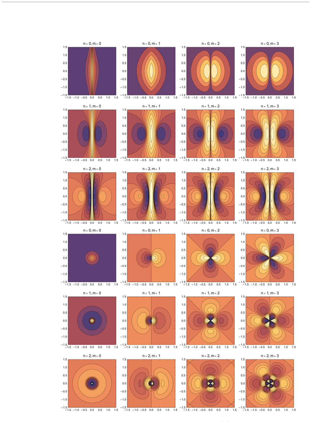
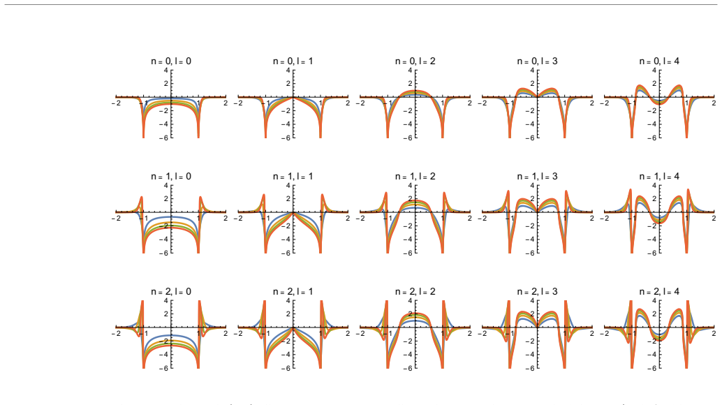
doi:10.1086/177404. arXiv:astro-ph/9601101 [astro-ph]. 23 Figure 4.Taking the well-known Hernquist and Ostriker (1992) results and transforming them according to (85) to produce ‘bisphericalised’ Hernquist-Ostriker density (top 3 rows) and potential (bottom 3 rows) basis functions, all viewed along they-axis. The indices shown aren=
work page internal anchor Pith review Pith/arXiv arXiv doi:10.1086/177404 1992
-
[4]
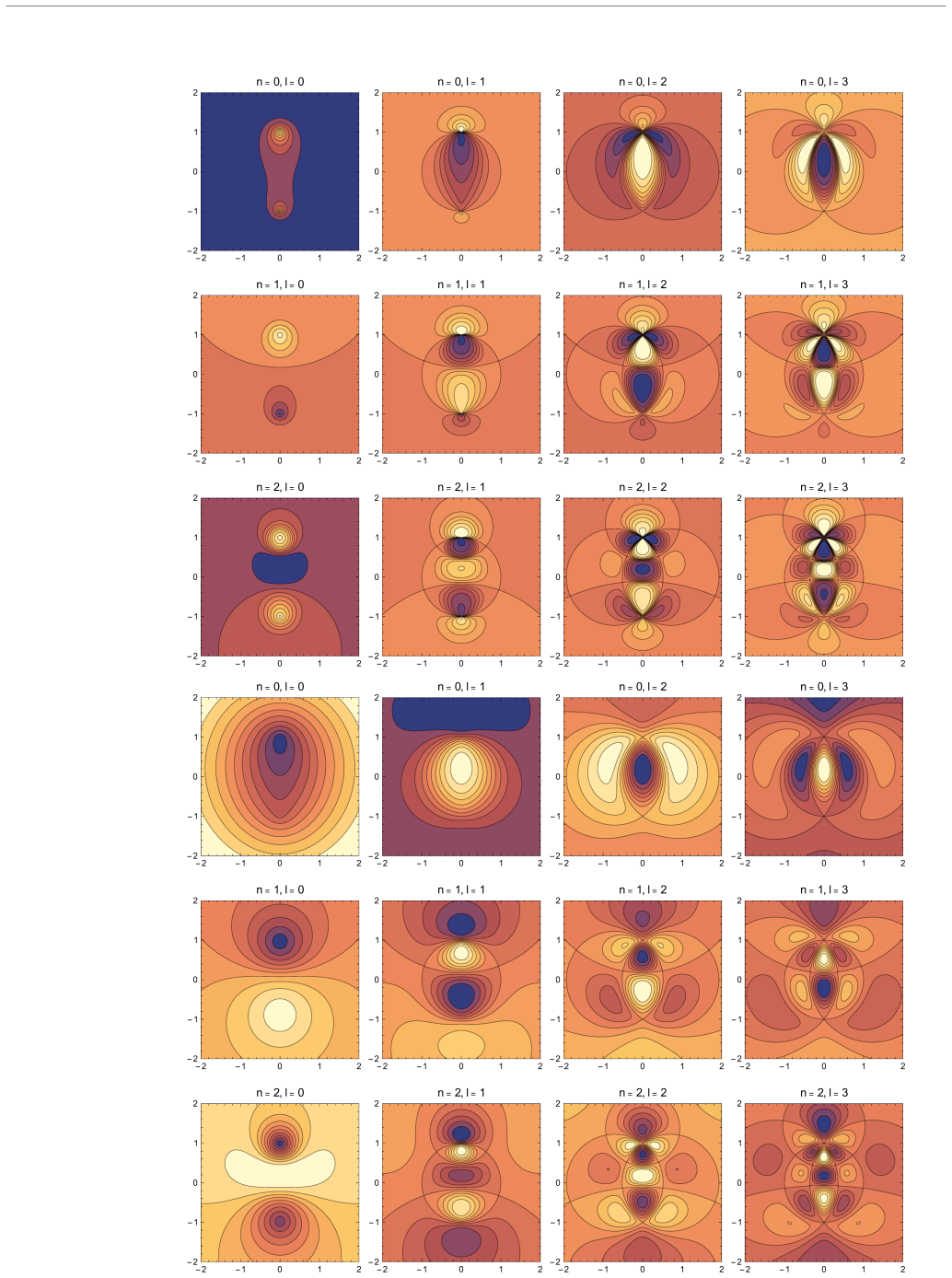
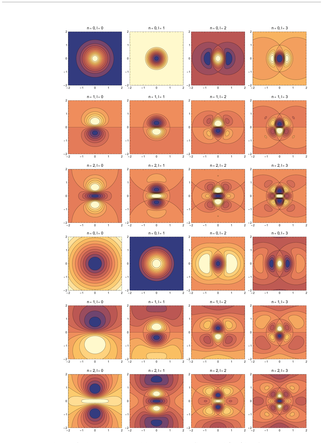
24 Figure 5.Similar to Fig. 4 but instead ‘bisphericalising’ the Clutton-Brock (1973) basis functions and choosing the parametersa=b= 1, producing a bispherical basis with an exact Plummer model as zeroth-order, but with bispherical higher order terms. Showing density (top 3 rows) and potential (bottom 3 rows) basis functions for n=
1973
-
[5]
Higher symmetries of the Laplacian
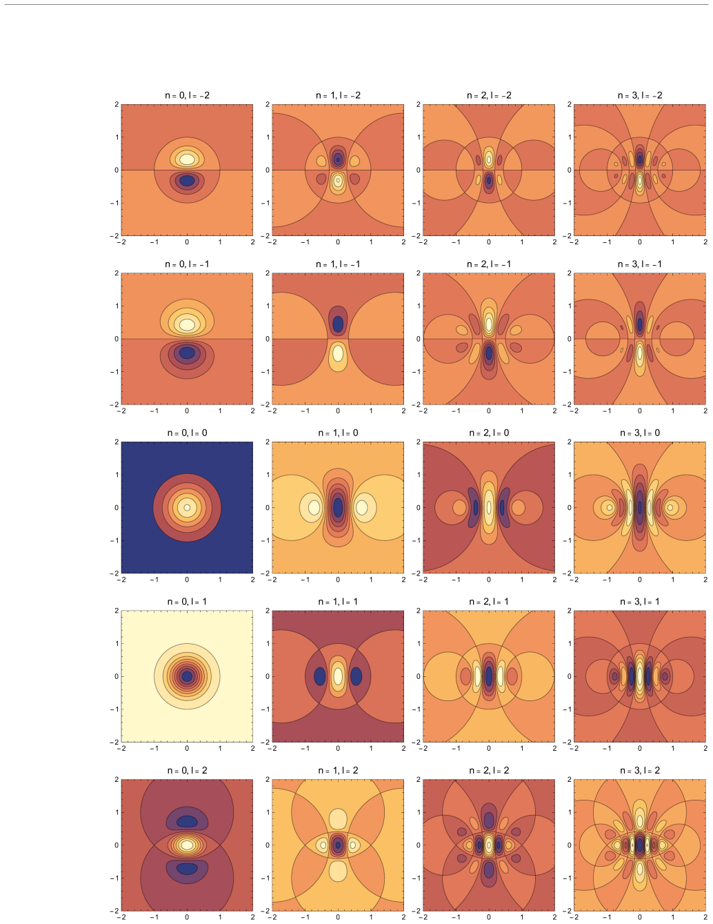
2 (across the page),l=−2. . .2 (down the page),m= 0 andb= 1, all viewed along they-axis. 26 Eastwood, Michael. “Higher symmetries of the Laplacian”. In:Annals of Mathematics161.3 (May 2005), pp. 1645–1665.issn: 0003-486X.doi:10 . 4007 / annals . 2005 . 161 . 1645.url:http : //dx.doi.org/10.4007/annals.2005.161.1645. Erd´ elyi, A. et al.Tables of integral ...
-
[6]
Computational Aspects of Orthogonal Polynomials
Gautschi, Walter. “Computational Aspects of Orthogonal Polynomials”. In:Orthogonal Polynomials. Springer Netherlands, 1990, pp. 181–216.isbn: 9789400905016.doi:10 . 1007 / 978 - 94 - 009 - 0501-6_9.url:http://dx.doi.org/10.1007/978-94-009-0501-6_9. — “Orthogonal polynomials—Constructive theory and applications”. In:Journal of Computational and Applied Mat...
-
[7]
Habashy, T. M., J. A. Kong, and W. C. Chew. “Scalar and vector Mathieu transform pairs”. In: Journal of Applied Physics60.10 (Nov. 1986), pp. 3395–3400.issn: 1089-7550.doi:10.1063/1. 337636.url:http://dx.doi.org/10.1063/1.337636. Hernquist, L. and J. P. Ostriker. “A self-consistent field method for galactic dynamics”. In:ApJ386 (Feb. 1992), pp. 375–397.do...
work page doi:10.1063/1 1986
-
[8]
Spectral properties of operators using tridiagonalisation
— “The structure and stability of self-gravitating disks”. In:MNRAS126 (Jan. 1963), p. 299.doi: 10.1093/mnras/126.4.299. Inayat-Hussain, A. A. “Mathieu integral transforms”. In:Journal of Mathematical Physics32.3 (Mar. 1991), pp. 669–675.issn: 1089-7658.doi:10.1063/1.529409.url:http://dx.doi.org/10. 1063/1.529409. Ismail, Mourad E. H. and Erik Koelink. “S...
work page internal anchor Pith review Pith/arXiv arXiv doi:10.1093/mnras/126.4.299 1963
-
[9]
A note on sampling expansion for a transform with parabolic cylinder kernel
Jerri, A. J. “A note on sampling expansion for a transform with parabolic cylinder kernel”. In: Information Sciences26.2 (Mar. 1982), pp. 155–158.issn: 0020-0255.doi:10 . 1016 / 0020 - 0255(82)90039-1.url:http://dx.doi.org/10.1016/0020-0255(82)90039-1. Jiang, Zhenglu and Leonid Ossipkov. “Two-integral distribution functions for axisymmetric stellar system...
-
[10]
301 pp. isbn: 978-0-7503-1314-8. Koelink, H. T. “On Jacobi and continuous Hahn polynomials”. In:Proceedings of the American Mathematical Society124.3 (1996), pp. 887–898.issn: 1088-6826.doi:10.1090/s0002- 9939- 96-03190-5. Koornwinder, Tom H. “Meixner–Pollaczek polynomials and the Heisenberg algebra”. In:Journal of Mathematical Physics30.4 (Apr. 1989), pp...
-
[11]
A two-parameter family of double-power-law biorthonormal potential-density expansions
—Basis Sets in Galactic Dynamics (PhD thesis). University of Cambridge, May 2020.url:https: //www.repository.cam.ac.uk/handle/1810/312444. Lilley, E. J., J. L. Sanders, and N. W. Evans. “A two-parameter family of double-power-law biorthonor- mal potential-density expansions”. In:MNRAS478 (July 2018), pp. 1281–1291.doi:10.1093/ mnras/sty1038. arXiv:1804.11...
work page internal anchor Pith review Pith/arXiv arXiv doi:10.1021/ct200115t.url:http: 2020
-
[12]
Navarro, J. F., C. S. Frenk, and S. D. M. White. “A Universal Density Profile from Hierarchical Clustering”. In:ApJ490 (Dec. 1997), pp. 493–508.doi:10.1086/304888. eprint:astro- ph/ 9611107. Naylor, D. “On an Integral Transform Involving a Class of Mathieu Functions”. In:SIAM Journal on Mathematical Analysis20.6 (Nov. 1989), pp. 1500–1513.issn: 1095-7154....
-
[13]
Biorthogonal Potential Density Sets for Flat Discs
Prudnikov, A.P., I.U.A. Brychkov, and O.I. Marichev.Integrals and Series Vols 1–3. Gordon and Breach Science Publishers, 1986.isbn: 9782881240904. Qian, Edward E. “Biorthogonal Potential Density Sets for Flat Discs”. In:MNRAS263 (July 1993), p. 394.doi:10.1093/mnras/263.2.394. — “Potential-density pairs for flat discs”. In:MNRAS257.4 (Aug. 1992), pp. 581–...
-
[14]
Rahmati, A. and M. A. Jalali. “New biorthogonal potential-density basis functions”. In:MNRAS 393 (Mar. 2009), pp. 1459–1466.doi:10.1111/j.1365-2966.2008.14226.x. arXiv:0811.1538. Reed, Michael and Barry Simon.Methods of Modern Mathematical Physics I: Functional Analysis: Volume
-
[15]
Potential-density basis sets in axisymmetric coordinates
Robijn, F. H. A. and David J. D. Earn. “Potential-density basis sets in axisymmetric coordinates”. In:MNRAS282.4 (Oct. 1996), pp. 1129–1142.doi:10.1093/mnras/282.4.1129. Saha, P. “Designer basis functions for potentials in galactic dynamics”. In:MNRAS262 (June 1993), pp. 1062–1064.doi:10.1093/mnras/262.4.1062. — “Unstable modes of a spherical stellar syst...
-
[16]
An adaptive algorithm for n-body field expansions
Tep, Kerwann, Christophe Pichon, and Michael S. Petersen. “Linear Response of Rotating and Flattened Stellar Clusters: The Oblate Kuzmin–Kutuzov St¨ ackel Family”. In:The Astrophysical Journal986.2 (June 2025), p. 203.issn: 1538-4357.doi:10 . 3847 / 1538 - 4357 / add5e5.url: http://dx.doi.org/10.3847/1538-4357/add5e5. Toomre, A. “On the Distribution of Ma...
work page internal anchor Pith review Pith/arXiv arXiv doi:10.3847/1538-4357/add5e5 2025
-
[17]
However, the decomposition of a generic second-order symmetry operator O= X i,j ci,j{Xi, Xj}+∇ 2f(97) is non-unique, as there exist 20 relations of the form O1 − O2 =∇ 2f1,2 (98) whereO 1 andO 2 are second-order operators andf 1,2 is a function, possibly zero. If we identify two operators (of any order) that differ byZ∇ 2 for some third operator or functi...
2005
-
[18]
In the simply separable caseu= 0 suffices, but we needu̸= 0 inR-separable coordinates
30 B Commutation ofT j We must find a functionusuch that the commutation relation [T ∗ 1 , T ∗ 2 ] = [gL1, gL2] + [g∇2, u] = 0 (104) holds. In the simply separable caseu= 0 suffices, but we needu̸= 0 inR-separable coordinates. Expanding out (104) we find that in general we must have u∝ 1 2 Z dq2 ∂1 log R2f1 ∂1∂2 logR 2 +∂ 2 1 ∂2 logR 2 ,(105) or equivalen...
1988
-
[19]
C Separable coordinates and conformal Killing tensors The classification ofR-separable coordinate systems (Miller, 1984, Ch
the correct definition is u∝ 1 2 ∂2 1 logR 2 + 1 4 ∂1 log R2f1 2 − 1 2 q−2 2 .(106) These definitions ofuare essentially ad hoc, and a sounder theoretical basis would be desirable. C Separable coordinates and conformal Killing tensors The classification ofR-separable coordinate systems (Miller, 1984, Ch
1984
-
[20]
Given that these operatorsS j are already known, it would be convenient if we could construct our quasi-commuting operatorsT j out of them. Quasi-commuting operators (14) generically take the form T ∗ =D K +A∇ 2,(107) whereKis a symmetric conformal Killing tensor (CKT),Ais a self-adjoint operator, andD K is a canonical map between CKTs and differential op...
2005
-
[21]
Choosing the CKT part of eachT j according to the ansatz above, we have 49 T ∗ j =a jS1 +b jS2 +c j +h j∇2,(j= 1,2,3) (108) for some constants (aj, bj, cj) and functionsh j
In fact this ‘trivial’ approach accounts for all theT j considered in the present work, and on heuristic grounds it seems likely that this approach will also work for the remaining separable coordinate systems. Choosing the CKT part of eachT j according to the ansatz above, we have 49 T ∗ j =a jS1 +b jS2 +c j +h j∇2,(j= 1,2,3) (108) for some constants (aj...
1976
-
[22]
On the planez= 0 at zeroth order this reproduces the isochrone model, but away from the plane it is not in St¨ ackel form
n. On the planez= 0 at zeroth order this reproduces the isochrone model, but away from the plane it is not in St¨ ackel form. Comparison of thea= 0 (78) anda= 1 (114) cases would seem to suggest a simple formula for the intermediate values ofa, but this is stymied by the complicated form of (111) (of course, the intermediate cases can be produced numerica...
1973
-
[23]
Neither weight function appears to give classical polynomials, but the simple form ameliorates their numerical construction
which gives a weight function similar to (113) but containing an additional factor of|(l+3/2+iα) q|4; applying a similar operator toϱ (0) 0lm leads to a family of ‘scale-free’ power-law densities l/2 + 5/4 + i p T1/2 q 2 ϱ(0) 0lm = 2 ((l+|m|+ 1)/2) q+1 ((l+|m|+ 2)/2) q+1 sinh|m|η Ylm(ϑ, φ) πb2 coshl+|m|+3+2qη sinh2η+ sin 2ϑ , (116) whose weight function i...
1990
-
[24]
Coords:q 1 =η, q 2 =φ, q 3 =z, x=bcoshηcosφ, y=bsinhηsinφ h1 =−h 2 =b q cosh2η−cos 2 φ, f 1 =−f 2 =−h 3 =R= 1, g=b 2 cos2φ−cosh 2η Operators:L 1 =−g −1∂2 η, L 2 =−g −1∂2 φ, T ∗ 1 =−J 2 3 −b 2P2 1 −b 2 cosh2η∇2, T ∗ 2 =J 2 3 +b 2P2 1 +b 2 cos2φ∇2, T 3 =P 3 33 As in the cylindrical polar case we exchanged the roles of theφandzcoordinates. The eigen- potenti...
1986
-
[25]
Operators:L 1 =−g −1∂2 λ, L 2 =−g −1∂2 µ, T ∗ 1 ={J 3,P 2} −λ 2∇2, T ∗ 2 =−{J 3,P 2} −µ 2∇2, T 3 =P 3 Another cylindrical system. The eigenfunctions are ϕαβk(λ, µ, z) = −4π α2 +β 2 eikz Uα2/(2k) √ 2kλ Uβ2/(2k) √ 2kµ ,(120) Ψαβk(λ, µ, z) = −1 λ2 +µ 2 eikz Uα2/(2k) √ 2kλ Uβ2/(2k) √ 2kµ , whereU a(z) is a parabolic cylinder function (DLMF,§12); however the i...
1982
discussion (0)
Sign in with ORCID, Apple, or X to comment. Anyone can read and Pith papers without signing in.