Functional Equivalence in Attention: A Comprehensive Study with Applications to Linear Mode Connectivity
Pith reviewed 2026-06-27 01:35 UTC · model grok-4.3
The pith
Rotary positional encodings reduce the symmetry group of attention compared to sinusoidal ones, increasing expressivity.
A machine-rendered reading of the paper's core claim, the machinery that carries it, and where it could break.
Core claim
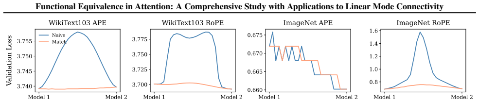
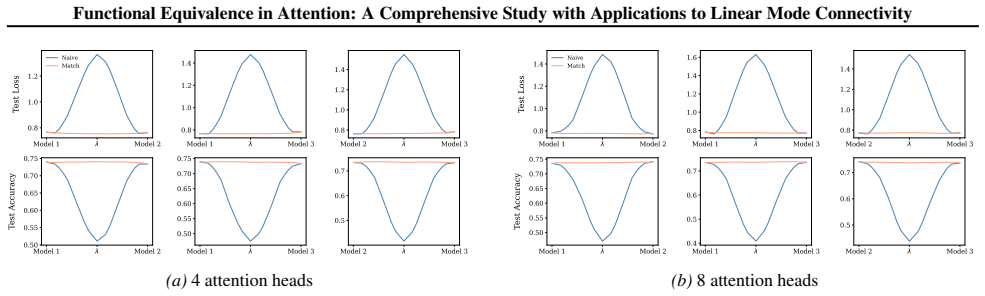
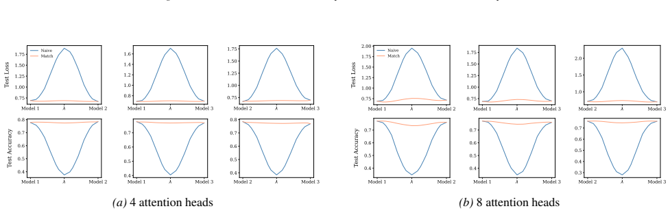
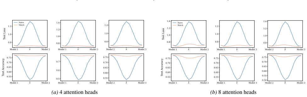
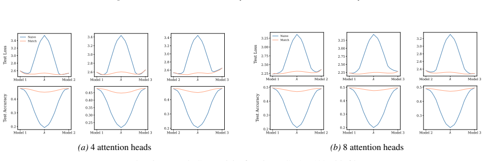
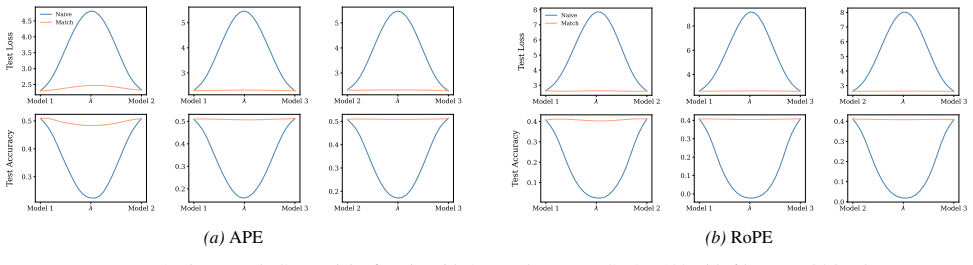
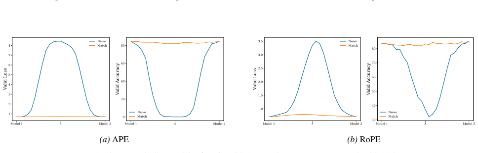
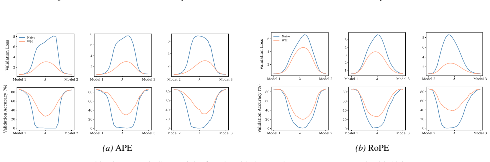
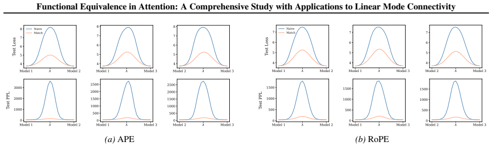
Focusing on the two most widely used variants—sinusoidal and rotary positional encodings—we show that sinusoidal encodings preserve the equivalence structure of vanilla attention, whereas rotary encodings significantly reduce the symmetry group, thereby enhancing expressivity. This offers a principled explanation for the growing prominence of RoPE in practice. We further examine how positional encodings affect linear mode connectivity, and through an alignment algorithm, empirically demonstrate that the presence and variability of connectivity across Transformer settings crucially depend on the positional encoding.
What carries the argument
The symmetry group of functional equivalence in multi-head attention under a given positional encoding; rotary encodings shrink this group relative to the sinusoidal or vanilla case.
If this is right
- Models using rotary encodings realize a larger set of distinct functions for any fixed parameter budget.
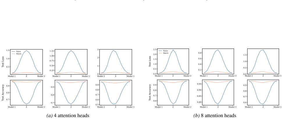
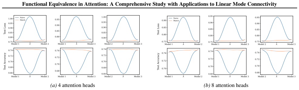
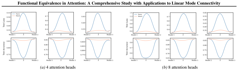
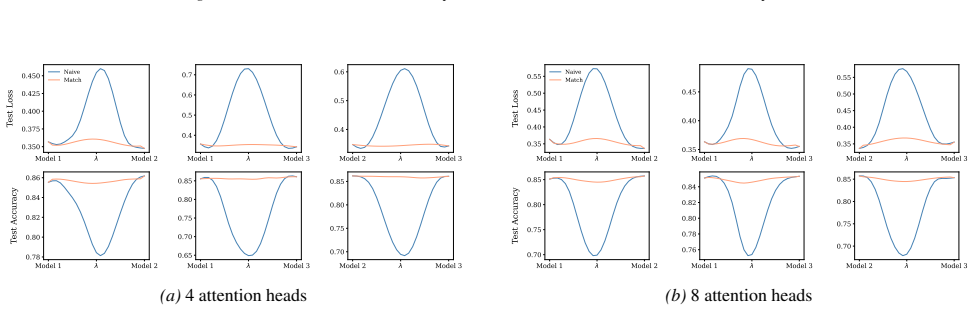
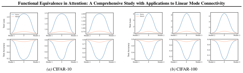
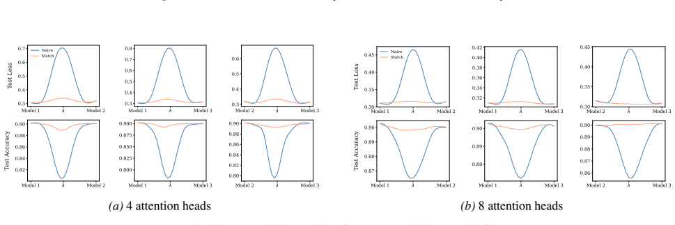
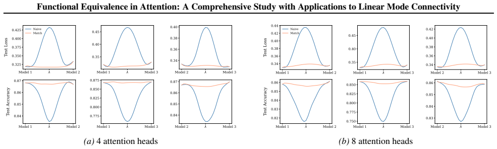
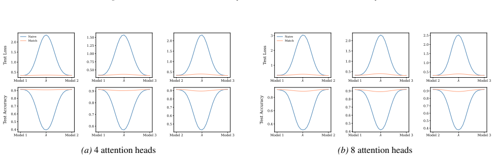
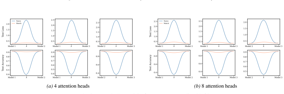
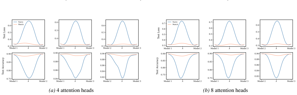
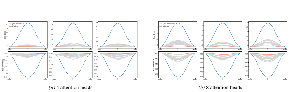
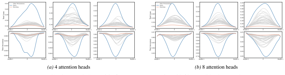
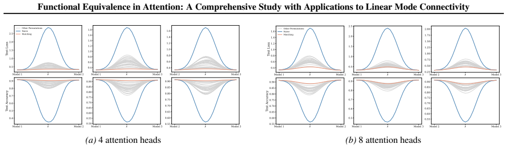
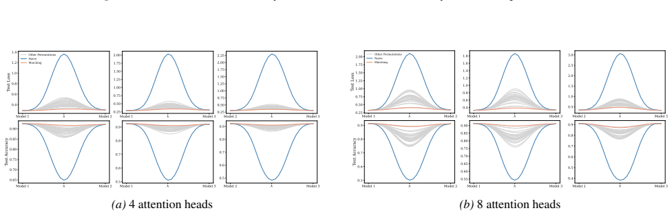
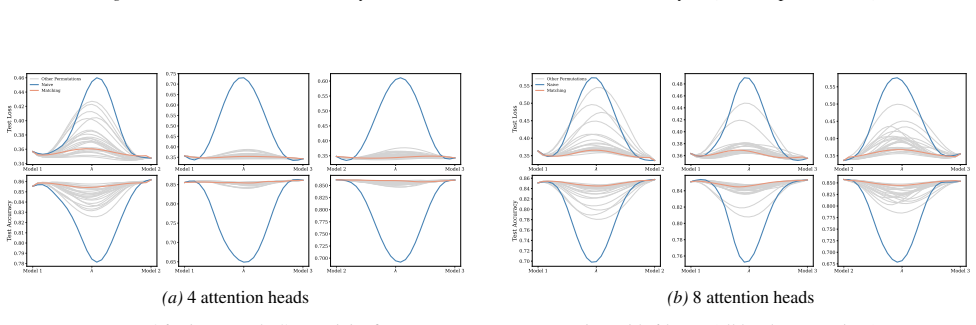
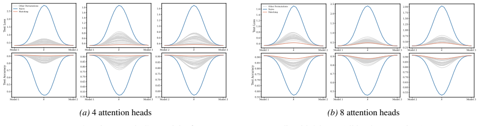
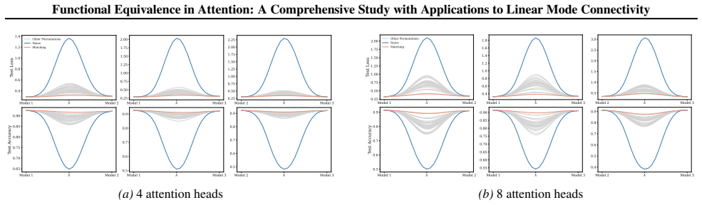
- Linear interpolation between independently trained models is more likely to produce high-loss points when rotary encodings are used.
- The choice of positional encoding directly controls how many parameter settings map to the same input-output behavior.
- Alignment procedures for finding connected modes must account for the encoding type to succeed.
Where Pith is reading between the lines
- The symmetry reduction may flatten or reshape the loss landscape in ways that improve optimization trajectories.
- The same analysis could be applied to other positional schemes such as ALiBi to predict their symmetry properties before empirical testing.
- Reduced equivalence might also affect the sample complexity needed to reach a given performance level.
Load-bearing premise
The formal analysis of equivalence is limited to the interaction between attention and the two chosen positional encodings and treats vanilla attention symmetries as the relevant baseline.
What would settle it
An explicit enumeration or group-order calculation that finds the same number of functionally distinct parameter configurations under rotary encodings as under sinusoidal encodings would refute the claimed reduction in symmetry group size.
Figures


read the original abstract
Neural network parameter spaces are inherently non-injective, as distinct parameter configurations can realize identical functions through functional equivalence. While this symmetry is well understood in classical fully connected and convolutional models, it becomes substantially more intricate in modern attention-based architectures. Existing analyses of multihead attention have largely focused on the vanilla formulation, overlooking positional encodings that fundamentally reshape architectural symmetries. In this work, we provide a formal study of functional equivalence in Transformers with positional encodings. Focusing on the two most widely used variants--sinusoidal and rotary positional encodings (RoPE)--we show that sinusoidal encodings preserve the equivalence structure of vanilla attention, whereas rotary encodings significantly reduce the symmetry group, thereby enhancing expressivity. This offers a principled explanation for the growing prominence of RoPE in practice. We further examine how positional encodings affect linear mode connectivity, and through an alignment algorithm, empirically demonstrate that the presence and variability of connectivity across Transformer settings crucially depend on the positional encoding.
Editorial analysis
A structured set of objections, weighed in public.
Referee Report
Summary. The paper provides a formal analysis of functional equivalence (symmetries) in multi-head attention, claiming that sinusoidal positional encodings preserve the equivalence structure of vanilla attention while rotary encodings (RoPE) reduce the size of the symmetry group and thereby increase expressivity. It further studies the consequences for linear mode connectivity (LMC) across Transformer variants and introduces an alignment algorithm to empirically demonstrate that connectivity patterns depend on the choice of positional encoding.
Significance. If the central claims hold, the work supplies a symmetry-based explanation for the empirical preference for RoPE and directly links architectural symmetries to the practical phenomenon of LMC. The combination of a formal symmetry analysis with an alignment-based empirical study of connectivity is a strength; the paper also supplies reproducible code for the alignment procedure.
major comments (2)
- [Formal analysis of attention with positional encodings] Formal analysis section (attention module only): the equivalence derivations and symmetry-group comparison are performed on the isolated attention block. The LMC experiments, however, are run on complete Transformer stacks that include layer norms, residual connections, and position-wise FFNs. No argument or ablation is given showing that the claimed reduction in symmetry group for RoPE survives these additional components; if the reduction is sensitive to the couplings, the headline claim that RoPE enhances expressivity via a smaller symmetry group does not necessarily transfer to the models studied in the connectivity experiments.
- [Linear mode connectivity experiments] LMC experiments and alignment algorithm: the paper asserts that connectivity 'crucially depend[s] on the positional encoding,' yet the reported results compare only sinusoidal versus RoPE without a controlled ablation that isolates the symmetry reduction from other architectural differences (e.g., different initialization or training schedules). A direct test—e.g., measuring connectivity after explicitly breaking or restoring the identified symmetries—would be needed to establish the causal link.
minor comments (2)
- Notation for the symmetry group and equivalence relation is introduced without a compact summary table; a single table listing the generators or orbit sizes for vanilla, sinusoidal, and RoPE cases would improve readability.
- [Abstract] The abstract states that the study is 'comprehensive,' yet only two positional-encoding families are treated; a brief discussion of why other common variants (e.g., ALiBi, learned embeddings) fall outside the scope would clarify the scope.
Simulated Author's Rebuttal
We thank the referee for the constructive feedback. The comments correctly identify that the formal analysis targets the attention module and that the LMC results rely on comparisons between two positional-encoding families. We address both points below and will revise the manuscript accordingly.
read point-by-point responses
-
Referee: [Formal analysis of attention with positional encodings] Formal analysis section (attention module only): the equivalence derivations and symmetry-group comparison are performed on the isolated attention block. The LMC experiments, however, are run on complete Transformer stacks that include layer norms, residual connections, and position-wise FFNs. No argument or ablation is given showing that the claimed reduction in symmetry group for RoPE survives these additional components; if the reduction is sensitive to the couplings, the headline claim that RoPE enhances expressivity via a smaller symmetry group does not necessarily transfer to the models studied in the connectivity experiments.
Authors: The symmetry analysis is performed on the attention block because that is the locus where positional encodings modify the functional equivalences between parameter configurations. Layer normalization, residual connections, and position-wise FFNs are equivariant with respect to the same parameter transformations (permutations for sinusoidal encodings, rotations for RoPE) that leave the attention output unchanged; consequently the reduced symmetry group identified for RoPE is expected to carry over to the full stack. We will add a short paragraph and a supporting remark in the revised manuscript making this invariance explicit and noting that an exhaustive ablation of every coupling lies outside the current scope. revision: yes
-
Referee: [Linear mode connectivity experiments] LMC experiments and alignment algorithm: the paper asserts that connectivity 'crucially depend[s] on the positional encoding,' yet the reported results compare only sinusoidal versus RoPE without a controlled ablation that isolates the symmetry reduction from other architectural differences (e.g., different initialization or training schedules). A direct test—e.g., measuring connectivity after explicitly breaking or restoring the identified symmetries—would be needed to establish the causal link.
Authors: All models in the LMC study share identical initialization distributions, optimizer settings, and training schedules; the sole controlled difference is the positional-encoding mechanism whose symmetry groups were derived in the formal section. The alignment procedure is constructed precisely to factor out the equivalences that remain under each encoding, and the observed connectivity patterns track the predicted group sizes. While an explicit symmetry-breaking intervention would constitute stronger causal evidence, such an experiment is not present in the current manuscript. We will expand the discussion to clarify the controls that were applied and to acknowledge that a direct interventional test remains future work. revision: partial
Circularity Check
Formal analysis of positional encoding symmetries is self-contained with no detected circularity
full rationale
The paper conducts a direct formal study of functional equivalence under sinusoidal and rotary positional encodings, comparing them to the vanilla attention baseline. No equations, fitted parameters, or predictions are shown that reduce by construction to the inputs (e.g., no self-definitional scaling, no fitted-input-called-prediction, no load-bearing self-citation chains). The central claims rest on explicit symmetry analysis rather than renaming or smuggling ansatzes. The empirical linear mode connectivity experiments are presented as separate demonstrations, not as forced outputs of the theoretical part. This matches the default expectation of non-circularity for theoretical architecture studies.
Axiom & Free-Parameter Ledger
Reference graph
Works this paper leans on
-
[3]
DeepSeek-V2: A Strong, Economical, and Efficient Mixture-of-Experts Language Model
doi: 10.18653/V1/P19-1285. URL https: //doi.org/10.18653/v1/p19-1285. DeepSeek-AI. Deepseek-v2: A strong, economi- cal, and efficient mixture-of-experts language model. CoRR, abs/2405.04434, 2024. doi: 10.48550/ARXIV . 2405.04434. URLhttps://doi.org/10.48550/ arXiv.2405.04434. DeepSeek-AI. Deepseek-r1: Incentivizing reasoning ca- pability in llms via rein...
work page internal anchor Pith review Pith/arXiv arXiv doi:10.18653/v1/p19-1285 2024
-
[4]
Draxler, F., Veschgini, K., Salmhofer, M., and Hamprecht, F
URL https://openreview.net/forum? id=YicbFdNTTy. Draxler, F., Veschgini, K., Salmhofer, M., and Hamprecht, F. A. Essentially no barriers in neural network energy landscape. In Dy, J. G. and Krause, A. (eds.),Proceed- ings of the 35th International Conference on Machine Learning, ICML 2018, Stockholmsm ¨assan, Stockholm, Sweden, July 10-15, 2018, volume 80...
2018
-
[5]
Du, S., Lee, J., Li, H., Wang, L., and Zhai, X
URL http://proceedings.mlr.press/ v80/draxler18a.html. Du, S., Lee, J., Li, H., Wang, L., and Zhai, X. Gradient descent finds global minima of deep neural networks. In International conference on machine learning, pp. 1675–
-
[6]
Entezari, R., Sedghi, H., Saukh, O., and Neyshabur, B
PMLR, 2019. Entezari, R., Sedghi, H., Saukh, O., and Neyshabur, B. The role of permutation invariance in linear mode con- nectivity of neural networks. InThe Tenth Interna- tional Conference on Learning Representations, ICLR 2022, Virtual Event, April 25-29, 2022. OpenReview.net,
2019
-
[7]
Fefferman, C
URL https://openreview.net/forum? id=dNigytemkL. Fefferman, C. and Markel, S. Recovering a feed-forward net from its output. In Cowan, J. D., Tesauro, G., and Alspec- tor, J. (eds.),Advances in Neural Information Processing Systems 6, [7th NIPS Conference, Denver, Colorado, USA, 1993], pp. 335–342. Morgan Kaufmann, 1993. Ferbach, D., Goujaud, B., Gidel, G...
1993
-
[8]
URL https://proceedings.mlr.press/ v238/ferbach24a.html. Frankle, J. Revisiting ”qualitatively characterizing neural network optimization problems”.CoRR, abs/2012.06898,
arXiv 2012
-
[9]
URL https://arxiv.org/abs/2012. 06898. Frankle, J. and Carbin, M. The lottery ticket hypothesis: Finding sparse, trainable neural networks. In7th Inter- national Conference on Learning Representations, ICLR 10 Functional Equivalence in Attention: A Comprehensive Study with Applications to Linear Mode Connectivity 2019, New Orleans, LA, USA, May 6-9, 2019....
2012
-
[10]
Using Mode Connectivity for Loss Landscape Analysis
PMLR, 2017. Gotmare, A., Keskar, N. S., Xiong, C., and Socher, R. Using mode connectivity for loss landscape analysis.CoRR, abs/1806.06977, 2018. URL http://arxiv.org/ abs/1806.06977. Guerrero-Pe˜na, F. A., Medeiros, H. R., Dubail, T., Aminbei- dokhti, M., Granger, E., and Pedersoli, M. Re-basin via implicit sinkhorn differentiation. InIEEE/CVF Confer- en...
work page internal anchor Pith review Pith/arXiv arXiv doi:10.1109/cvpr52729 2017
-
[11]
Keskar, N
URL https://openreview.net/forum? id=UqYNPyotxL. Keskar, N. S., Mudigere, D., Nocedal, J., Smelyanskiy, M., and Tang, P. T. P. On large-batch training for deep learn- ing: Generalization gap and sharp minima. In5th Inter- national Conference on Learning Representations, ICLR 2017, Toulon, France, April 24-26, 2017, Conference Track Proceedings. OpenReview...
2017
-
[12]
In: IEEE/CVF Conference on Computer Vision and Pattern Recognition Workshops (CVPRW), pp 3347–3356
URL https://openreview.net/forum? id=cUFIil6hEG. Kozal, J., Wasilewski, J., Krawczyk, B., and Wozniak, M. Continual learning with weight interpolation. In IEEE/CVF Conference on Computer Vision and Pattern Recognition, CVPR 2024 - Workshops, Seattle, WA, USA, June 17-18, 2024, pp. 4187–4195. IEEE, 2024. doi: 10.1109/CVPRW63382.2024.00422. URL https:// doi...
-
[13]
URL https: //doi.org/10.1162/neco.1994.6.3.543
doi: 10.1162/NECO.1994.6.3.543. URL https: //doi.org/10.1162/neco.1994.6.3.543. LeCun, Y ., Bottou, L., Bengio, Y ., and Haffner, P. Gradient- based learning applied to document recognition.Proc. IEEE, 86(11):2278–2324, 1998. doi: 10.1109/5.726791. URLhttps://doi.org/10.1109/5.726791. Lehmann, J., Isele, R., Jakob, M., Jentzsch, A., Kontokostas, D., Mende...
-
[14]
Pittorino, F., Ferraro, A., Perugini, G., Feinauer, C., Bal- dassi, C., and Zecchina, R
URL https://openreview.net/forum? id=Bylx-TNKvH. Pittorino, F., Ferraro, A., Perugini, G., Feinauer, C., Bal- dassi, C., and Zecchina, R. Deep networks on toroids: Removing symmetries reveals the structure of flat re- gions in the landscape geometry. In Chaudhuri, K., Jegelka, S., Song, L., Szepesv ´ari, C., Niu, G., and Sabato, S. (eds.),International Co...
2022
-
[15]
URL https://proceedings.mlr.press/ v162/pittorino22a.html. Piziak, R. and Odell, P. L. Full rank factorization of matrices. Mathematics magazine, 72(3):193–201, 1999. Press, O., Smith, N. A., and Lewis, M. Train short, test long: Attention with linear biases enables input length extrapolation. InThe Tenth International Conference on Learning Representatio...
-
[17]
Vlaar, T
URL https://jmlr.org/papers/v20/ 18-674.html. Vlaar, T. J. and Frankle, J. What can linear interpolation of neural network loss landscapes tell us? In Chaud- huri, K., Jegelka, S., Song, L., Szepesv ´ari, C., Niu, G., and Sabato, S. (eds.),International Conference on Ma- chine Learning, ICML 2022, 17-23 July 2022, Balti- more, Maryland, USA, volume 162 of...
2022
-
[18]
Wen, H., Cheng, H., Qiu, H., Wang, L., Pan, L., and Li, H
URL https://proceedings.mlr.press/ v162/vlaar22a.html. Wen, H., Cheng, H., Qiu, H., Wang, L., Pan, L., and Li, H. Optimizing mode connectivity for class incremental learn- ing. In Krause, A., Brunskill, E., Cho, K., Engelhardt, B., Sabato, S., and Scarlett, J. (eds.),International Con- ference on Machine Learning, ICML 2023, 23-29 July 2023, Honolulu, Haw...
2023
-
[19]
URL https://proceedings.mlr.press/ v162/wortsman22a.html. Xiao, T. Z., Liu, W., and Bamler, R. A compact repre- sentation for bayesian neural networks by removing per- mutation symmetry.CoRR, abs/2401.00611, 2024. doi: 10.48550/ARXIV .2401.00611. URL https://doi. org/10.48550/arXiv.2401.00611. Yang, A., Li, A., Yang, B., Zhang, B., Hui, B., Zheng, B., Yu,...
work page internal anchor Pith review doi:10.48550/arxiv 2024
-
[20]
Functional Equivalence in Attention: A Comprehensive Study with Applications to Linear Mode Connectivity
URL https://openreview.net/forum? id=SJgwzCEKwH. Zheng, C., Gao, Y ., Shi, H., Huang, M., Li, J., Xiong, J., Ren, X., Ng, M. K., Jiang, X., Li, Z., and Li, Y . DAPE: data-adaptive positional encoding for length extrapola- tion. In Globersons, A., Mackey, L., Belgrave, D., Fan, A., Paquet, U., Tomczak, J. M., and Zhang, C. (eds.), Advances in Neural Inform...
2024
-
[21]
Related concepts, such as functional equivalence and alignment methods, are also introduced in connection with prior literature
Section 1 provides an introduction and related work on Linear Mode Connectivity. Related concepts, such as functional equivalence and alignment methods, are also introduced in connection with prior literature
-
[22]
Section 2 reviews vanilla attention, including its parameter space, symmetry group, and a result from literature– Theorem 2.1–which establishes complete functional equivalence for vanilla attention
-
[23]
While absolute PEs of the additive type do not affect the structure, relative PEs (with particular emphasis on Rotary PE) fundamentally change the attention mechanism
Section 3 examines how positional encodings may alter the internal structure of attention, thereby rendering the analysis from the vanilla case no longer directly applicable. While absolute PEs of the additive type do not affect the structure, relative PEs (with particular emphasis on Rotary PE) fundamentally change the attention mechanism. The correspond...
-
[24]
First, we extend the RoPE setting to a general attention formulation that accommodates all cases of interest
Section 4 focuses primarily on the RoPE case. First, we extend the RoPE setting to a general attention formulation that accommodates all cases of interest. In this formulation, the similarity score between two tokens at their specific positional indices is expressed as a bilinear form or quadratic norm. The result on functional equivalence of this setting...
-
[25]
We propose a two-stage alignment algorithm for multi-head attention layers, applicable to both standard MHA and MHA with RoPE
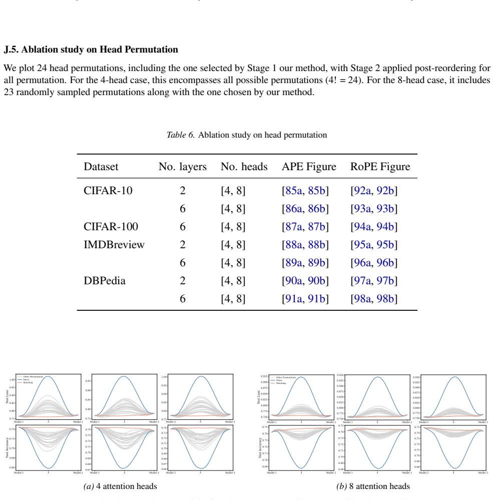
Section 5 introduces an alignment method that serves as a tool for examining linear mode connectivity (LMC) in attention-based models. We propose a two-stage alignment algorithm for multi-head attention layers, applicable to both standard MHA and MHA with RoPE. The first stage matches the ordering of attention heads between two models by solving a linear ...
-
[26]
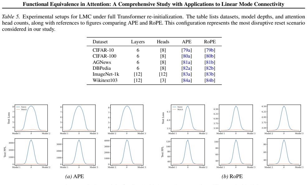
Experiments are conducted across diverse Vision and NLP tasks
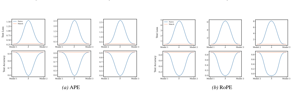
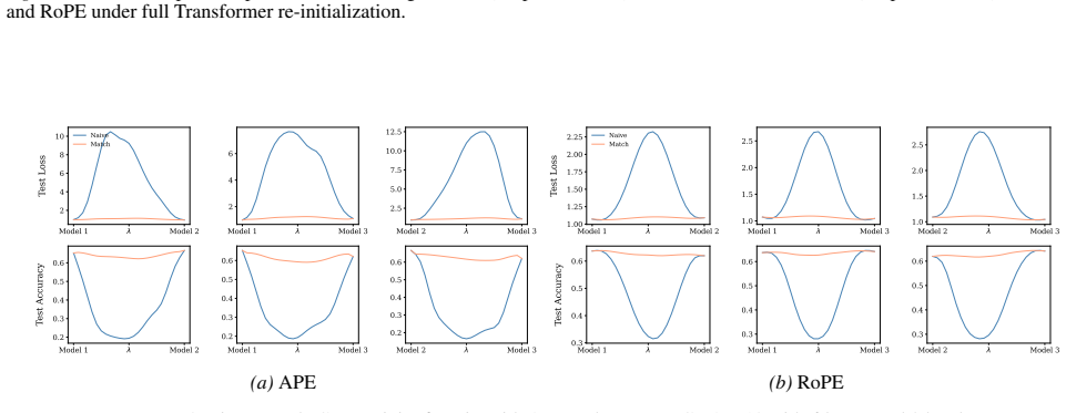
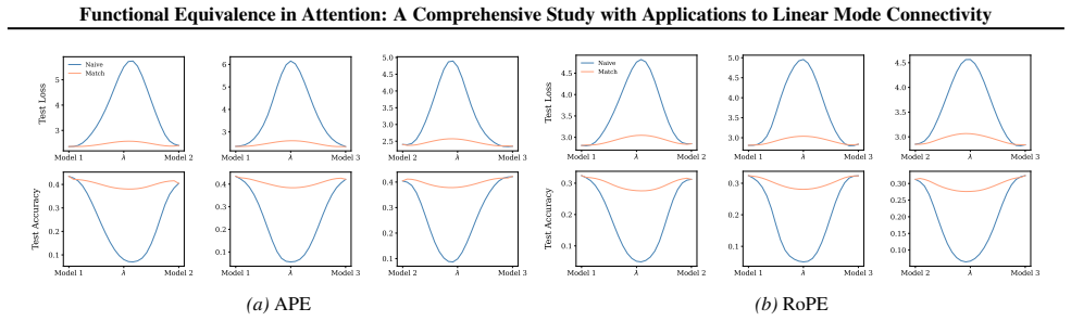
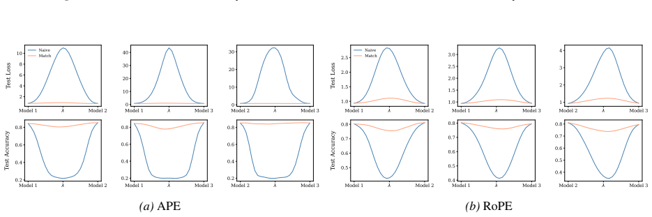
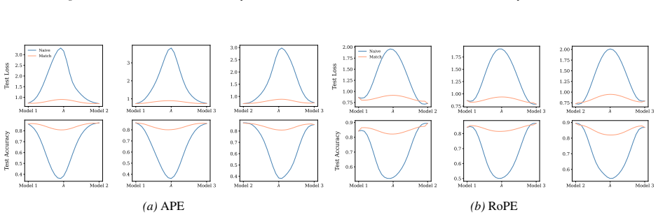
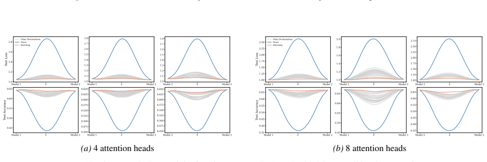
Section 6 examines LMC under four re-initialization strategies, with emphasis on the first attention layer and full model resets, while intermediate cases are reported in the Appendix. Experiments are conducted across diverse Vision and NLP tasks. Ablation studies confirm the effectiveness of the two-stage matching algorithm in reducing barriers: Ablation...
-
[27]
Section 7 summarizes our findings, discusses limitations, and outlines future directions. 18 Functional Equivalence in Attention: A Comprehensive Study with Applications to Linear Mode Connectivity Appendix.The appendices provide complete proofs of the theoretical results in the main paper, the proposed matching algorithms, as well as additional experimen...
-
[28]
Appendix B formally defines the attention mechanism and its parameter space, followed by a description of how positional encodings are incorporated into attention
-
[29]
Appendix C briefly describes the symmetry structures of vanilla attention, attention with absolute PEs, and attention with relative PEs (with emphasis on RoPE)
-
[30]
Theorem D.1, which is Theorem 4.1 in the main paper, establishes the functional equivalence of this general setting
Appendix D introduces the general attention formulation. Theorem D.1, which is Theorem 4.1 in the main paper, establishes the functional equivalence of this general setting. The proof can be sketched as follows: starting from the softmax operator, we multiply through the denominators to rewrite the expression as an exponential polynomial, and then apply r...
-
[31]
Theorem F.1, corresponding to Theorem 4.2 in the main paper, provides the full details of this analysis
Appendix F applies the functional equivalence analysis of the general attention case to the specific setting of RoPE. Theorem F.1, corresponding to Theorem 4.2 in the main paper, provides the full details of this analysis. The proof proceeds as follows: RoPE is first reformulated as a special case of the general attention formulation via reparameterizatio...
-
[32]
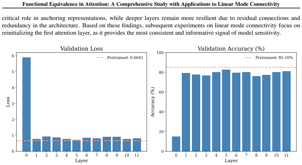
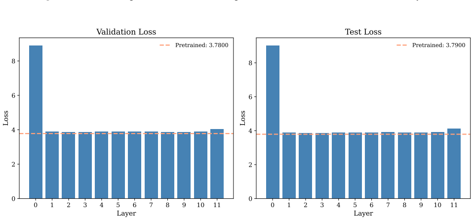
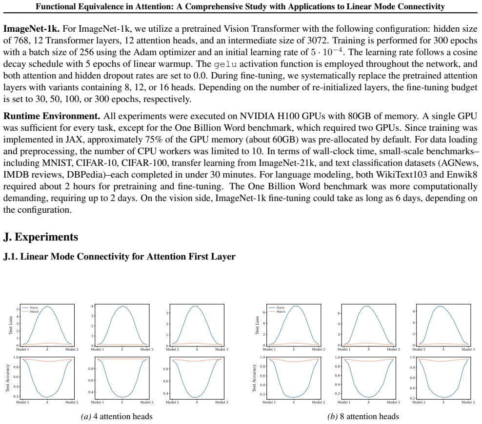
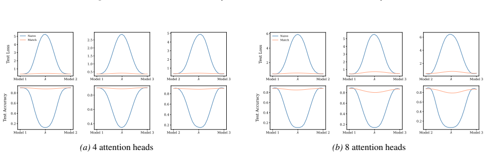
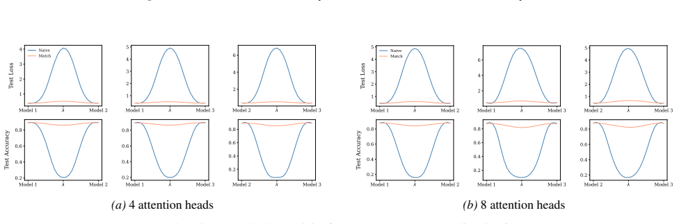
Appendix J.1 reports experiments on re-initializing only the first attention layer, highlighting its dominant role in shaping early representations
-
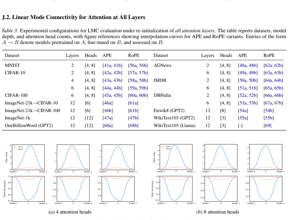
[33]
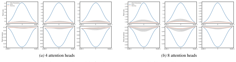
Appendix J.2 investigates re-initialization of all attention layers, showing the cumulative effect of disrupting contextual interactions across the network
-
[34]
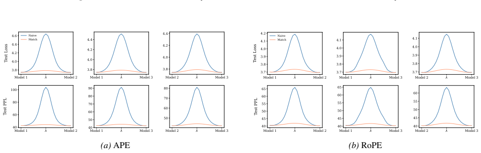
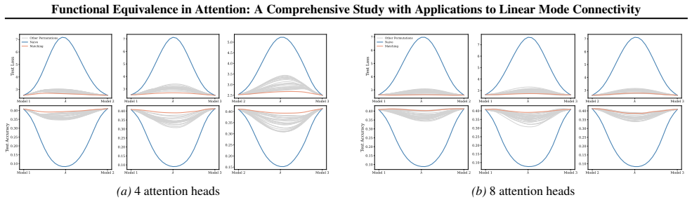
Appendix J.3 studies re-initialization of the first Transformer layer, coupling attention and its adjacent feedforward block to examine early-layer sensitivity
-
[35]
19 Functional Equivalence in Attention: A Comprehensive Study with Applications to Linear Mode Connectivity
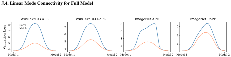
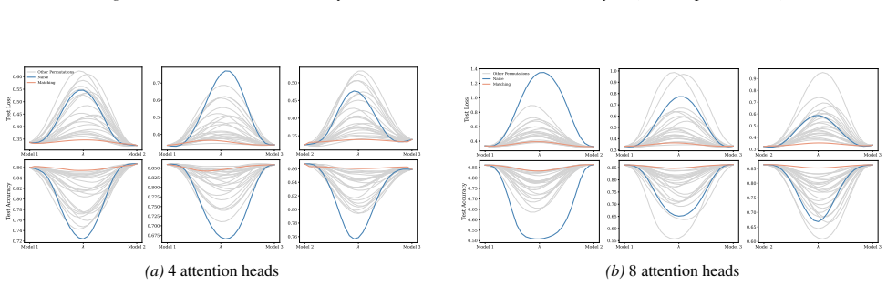
Appendix J.4 evaluates the most extreme setting where the entire Transformer is re-initialized, quantifying the magnitude of barriers introduced by full resets. 19 Functional Equivalence in Attention: A Comprehensive Study with Applications to Linear Mode Connectivity
-
[36]
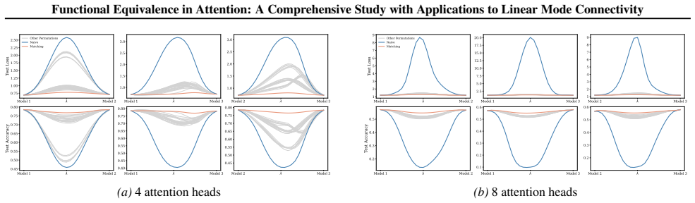
Appendix J.5 presents ablation studies on head permutation, including the two-stage matching algorithm. Stage 1 demonstrates the necessity of optimal head alignment for preserving linear mode connectivity, while Stage 2 leverages gradient refinement to further reduce interpolation barriers. The experimental findings indicate that linear mode connectivity ...
2017
-
[37]
Everyd×d h matrix appearing inθand ¯θhas full column rankd h
-
[38]
If the twoMHAmaps are identical, thenh= ¯h, and there existsg∈G Att(dh, h)such that ¯θ=gθ
Thehmatrices{W Q i (W K i )⊤}h i=1 are pairwise distinct; and, the ¯hmatrices{ ¯W Q i ( ¯W K i )⊤}¯h i=1 are pairwise distinct. If the twoMHAmaps are identical, thenh= ¯h, and there existsg∈G Att(dh, h)such that ¯θ=gθ. Remark C.2.While the theorem imposes certain assumptions on the parameters of the MHA maps, it is important to emphasize that these condit...
-
[39]
(Relative positional encoding assumption.) For allm, n≥1and for all shiftsk≥0, we assume Am,n =A m+k,n+k.(33) This corresponds to the natural stationarity condition imposed by relative positional encodings
-
[40]
(Diagonal self-similarity terms are symmetric.) For each m≥1 , the matrix Am,m i parameterizes the function f that computes the similarity score of the m-th token with itself at the i-th head, namely xmAm,m i x⊤ m. Since every quadratic form corresponds uniquely to a symmetric matrix, we may, without loss of generality, symmetrizeA m,m i : sym(Am,m i ) :=...
-
[41]
In particular, we note that it suffices to show that at least one of the coefficientsBi must vanish
Preliminary setup.We first record some initial observations and introduce the necessary notation in preparation for the proof. In particular, we note that it suffices to show that at least one of the coefficientsBi must vanish. Once this is established, symmetry in the construction allows us to conclude that in fact all Bi must be equal to zero, thereby p...
-
[42]
Specifically, the symmetry conditions imposed by the Ak,t i on admissible permutations force the Bi to satisfy a family of linear relations indexed by i∈[h]
Structural constraints on the Bi.By applying the above linear independence principle, we identify a fundamental structural constraint on the coefficients Bi. Specifically, the symmetry conditions imposed by the Ak,t i on admissible permutations force the Bi to satisfy a family of linear relations indexed by i∈[h] . These constraints form the core of the a...
-
[43]
This step is preparatory: it shows that the relations identified in the previous step are not only necessary but also sufficient to deduce that at least one Bi must vanish
Partition-based refinement.We next examine the equalities that occur within the sets of h elements {Ak,t i }h i=1. This step is preparatory: it shows that the relations identified in the previous step are not only necessary but also sufficient to deduce that at least one Bi must vanish. The analysis exploits the partition structure {Up}, together with the...
-
[44]
The linear relations obtained inStep 3, when applied to the partition refinement ofStep 4, imply that one of the Bi’s must equal zero
Conclusion.Finally, we combine the above ingredients to conclude the proof. The linear relations obtained inStep 3, when applied to the partition refinement ofStep 4, imply that one of the Bi’s must equal zero. By the initial reduction inStep 1, this suffices to deduce that in fact allB i = 0. This completes the proof of the theorem. We proceed to present...
-
[45]
In particular, by reindexing the head indices, we may assume U1 ={1,
For all t∈S , the partition {U t p}αt p=1, defined inStep 4, coincides with {Up}α p=1. In particular, by reindexing the head indices, we may assume U1 ={1, . . . , m}. This guarantees that the structure of the partition is stable across infinitely manyt∈S, providing us with a consistent reference framework
-
[46]
For all ti with i∈[γ] , where γ < m , recall that V ti =U ti(1)∩ {1, . . . , m} . One can select γ head indices vi ∈V ti such that they are pairwise distinct. This property will be crucial later when we need to ensure that certain representatives can be chosen without overlap. We also recall the main result fromStep 3, namely Equation (57): for any (s1, ....
-
[47]
In other words, the positions corresponding to T are aligned with the distinguished token indicest i
If j=v i for some i∈T , then set sj =s vi =t i. In other words, the positions corresponding to T are aligned with the distinguished token indicest i
-
[48]
, m} \ {v i :i∈T} , take sj to be an arbitrary element of S
If j∈ {1, . . . , m} \ {v i :i∈T} , take sj to be an arbitrary element of S. This ensures consistency with the partition structure while leaving us flexibility in the assignment
-
[49]
Again, this choice respects the partitioning of indices into classesU p
If j∈U p for some 2≤p≤α , then take sj to be an arbitrary element of S. Again, this choice respects the partitioning of indices into classesU p. For the chosen (s1, . . . , sh)∈[L] h, we analyze which σ∈S h satisfy the condition Ak,sj j =A k,sj σ(j) for all j∈[h] . We make the following observations, case by case:
-
[50]
Hence σ(U2 ⊔U 3 ⊔ · · · ⊔U α) =U 2 ⊔U 3 ⊔ · · · ⊔U α,(69) and consequentlyσ(U 1) =U 1
Forj∈U 2 ⊔U 3 ⊔ · · · ⊔U α, sayj∈U p with2≤p≤α, the conditionA k,sj j =A k,sj σ(j) impliesσ(j)∈U p. Hence σ(U2 ⊔U 3 ⊔ · · · ⊔U α) =U 2 ⊔U 3 ⊔ · · · ⊔U α,(69) and consequentlyσ(U 1) =U 1. In particular, ifj∈U 1, thenσ(j)∈U 1
-
[51]
, m} \ {v i :i∈T} , if Ak,sj j =A k,sj σ(j), then necessarily σ(j)∈U 1 ={1,
For j∈ {1, . . . , m} \ {v i :i∈T} , if Ak,sj j =A k,sj σ(j), then necessarily σ(j)∈U 1 ={1, . . . , m} . Thus the entire set U1 is stable underσ, but the specific images of these indices may vary withinU 1
-
[52]
From the previous point, we also know σ(j)∈U 1
For j=v i with i∈T , if Ak,sj j =A k,sj σ(j), then σ(j)∈U svi (1) =U ti(1). From the previous point, we also know σ(j)∈U 1. Taken together, these conditions imply that σ(j)∈V ti =U ti(1)∩U 1. In other words, the image of vi underσis constrained to lie inside the restricted setV ti. Therefore, specifying aσ∈S h that satisfiesA k,sj j =A k,sj σ(j) for allj∈...
-
[53]
For eachj=v i withi∈T, choosingσ(j) =σ(v i)∈V ti,
-
[54]
, m} \ {v i :i∈T}, choosingσ(j)∈U 1 \ {σ(vi) :i∈T}arbitrarily,
For eachj∈ {1, . . . , m} \ {v i :i∈T}, choosingσ(j)∈U 1 \ {σ(vi) :i∈T}arbitrarily,
-
[55]
In conclusion, the structure of admissible permutations σ in Equation (67) is fully determined by the subset T⊂[γ] and the representatives vi ∈V ti chosen inStep 4
For eachj∈U p with2≤p≤α, choosingσ(j)∈U p. In conclusion, the structure of admissible permutations σ in Equation (67) is fully determined by the subset T⊂[γ] and the representatives vi ∈V ti chosen inStep 4. This description clarifies how the constraints arising from the partition classes Up and the distinguished representatives vi together restrict the a...
1935
-
[56]
All matricesA n i and ¯An i , for feasibleiandn∈Z, are nonzero
-
[57]
,{An h}n∈Z are pairwise distinct
Fromθ, thehfamilies{A n 1 }n∈Z, . . . ,{An h}n∈Z are pairwise distinct. The same condition holds for ¯θ
-
[58]
If the twoMHA RoPE maps are identical, thenh= ¯h
All matricesW Q i , W K i , W V i , W O i and ¯W Q i , ¯W K i , ¯W V i , W O i , for feasiblei, are of rankd h. If the twoMHA RoPE maps are identical, thenh= ¯h. Moreover, there existsg∈G RoPE(dh, h)such that ¯θ=gθ. Proof.Fori∈[h]andm, n≥1, defineA m,n i =A m−n i andB i :=W V i (W O i )⊤. Same for ¯Am,n i and ¯Bi. Then, one has MHA x;{{A m,n i }m,n, Bi}h ...
1999
-
[59]
Compute the scalar constantsη Q, ηK and the complex constantsγ Q, γK
-
[60]
Define the objective functiong(x) =xη Q + ηK x −4 q |γQ|2x+ |γK |2 x + 2Re(γQ¯γK)
-
[61]
Here we use the Brent’s method (Brent, 2013)
Find the minimizer x⋆ = arg min x>0 g(x) using a numerical optimization routine. Here we use the Brent’s method (Brent, 2013). The optimal solution is computed as r⋆ = √ x⋆, θ⋆ =−arg r⋆γQ + 1 r⋆ γK , and finally a=r ⋆ cos(θ⋆),b=r ⋆ sin(θ⋆). This yields the optimal alignment matrixU j for each subspacej. G.2. Algorithm Description Algorithm 1Attention Laye...
2013
-
[62]
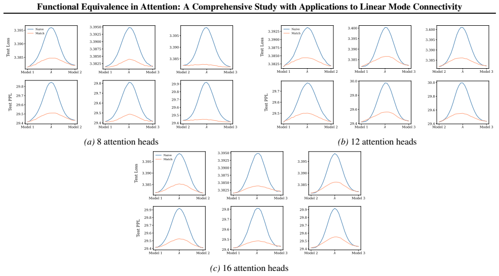
During fine-tuning, we replace the pretrained attention modules with variants containing 4, 8, or 16 heads, and train for 60000 steps
Pretraining is performed using the Adam optimizer with a batch size of 24 and an initial learning rate of 2.5·10 −4, following a cosine decay schedule without warmup, for a total of 60000 steps. During fine-tuning, we replace the pretrained attention modules with variants containing 4, 8, or 16 heads, and train for 60000 steps. WikiText103.For the WikiTex...
2000
discussion (0)
Sign in with ORCID, Apple, or X to comment. Anyone can read and Pith papers without signing in.