Enhancing neural network extrapolation in thermo-fluid systems using steady-state solutions
Pith reviewed 2026-06-26 21:37 UTC · model grok-4.3
The pith
A neural network ansatz that decomposes solutions into a prescribed steady state plus a decaying transient correction embeds long-time convergence by construction for dissipative PDEs.
A machine-rendered reading of the paper's core claim, the machinery that carries it, and where it could break.
Core claim
The proposed ansatz decomposes the solution into a steady-state component and a transient correction modulated by a time-dependent decay profile. When the decay profile vanishes at long time and the transient correction remains bounded, the representation embeds convergence to the prescribed steady state directly into the architecture rather than enforcing it through an additional penalty term. This allows the network to learn the transient dynamics while preserving the correct asymptotic behavior.
What carries the argument
The steady-state-informed ansatz that writes the solution as the sum of a prescribed steady-state field and a bounded transient correction multiplied by a decay profile that vanishes at large times.
If this is right
- The network only needs to learn the transient correction; the long-time limit is satisfied automatically by the functional form.
- Temporal extrapolation beyond the training interval improves compared with networks that lack the explicit asymptotic embedding.
- The approach applies to dissipative systems ranging from the one-dimensional heat equation to incompressible Navier-Stokes flow and three-dimensional conjugate heat transfer.
- Training uses the physics-informed loss inside a PINN framework without an additional steady-state penalty.
Where Pith is reading between the lines
- The same decomposition could be tried on systems whose steady states are computed once by a separate solver and then frozen for the network.
- If the decay profile itself is learned rather than prescribed, the method might adapt to cases where the relaxation rate is not known in advance.
- The construction may reduce the amount of long-time data needed during training because the network is not free to drift away from the known equilibrium.
Load-bearing premise
The PDE solutions relax toward a stationary equilibrium that can be prescribed or computed independently and supplied to the network.
What would settle it
A numerical example in which the learned transient correction grows unbounded even though the decay profile vanishes would show that the architectural guarantee of convergence does not hold.
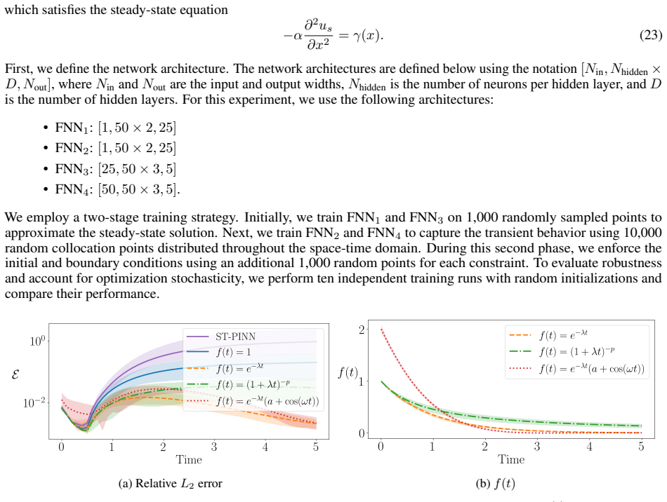
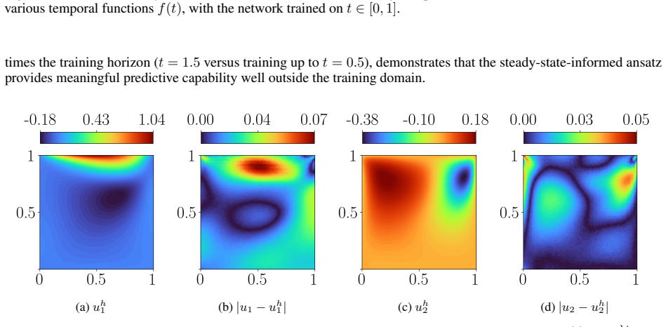
Figures


read the original abstract
Time-dependent partial differential equations (PDEs) arise in many engineering systems, including thermo-fluid applications. Classical numerical simulations of such systems can become computationally expensive for long-time dynamics because they typically require sequential time integration with time steps constrained by stability, accuracy, or nonlinear solvers. Although scientific machine learning provides an alternative for approximating PDE solutions, standard neural network approximations often degrade when extrapolated beyond the training time interval. In this work, we propose a steady-state-informed neural network representation for dissipative PDE systems whose solutions relax toward a stationary equilibrium. The proposed ansatz decomposes the solution into a steady-state component and a transient correction modulated by a time-dependent decay profile. When the decay profile vanishes at long time and the transient correction remains bounded, the representation embeds convergence to the prescribed steady state directly into the architecture, rather than enforcing it through an additional penalty term. This allows the network to learn the transient dynamics while preserving the correct asymptotic behavior. We implement the approach within a physics-informed neural network (PINN) framework and train the resulting model using the SOAP optimizer. The method is evaluated on a sequence of problems of increasing physical and geometric complexity, ranging from the one-dimensional heat equation to incompressible Navier-Stokes flow in a lid-driven cavity, natural convection in a square cavity, and a full three-dimensional conjugate heat transfer problem. The numerical results show that the steady-state-informed architecture substantially improves temporal extrapolation beyond the training interval compared with architectures that do not explicitly enforce the asymptotic condition.
Editorial analysis
A structured set of objections, weighed in public.
Referee Report
Summary. The paper proposes a steady-state-informed neural network ansatz for dissipative time-dependent PDEs whose solutions relax to a stationary equilibrium. The solution is decomposed as a prescribed steady-state component plus a neural-network-modeled transient correction modulated by a decay profile that vanishes at long times. When the transient remains bounded, this embeds asymptotic convergence directly into the architecture rather than via an added penalty. The ansatz is implemented in a PINN framework trained with the SOAP optimizer and evaluated on a sequence of problems of increasing complexity (1D heat equation, lid-driven cavity, natural convection, 3D conjugate heat transfer), with the claim that it substantially improves temporal extrapolation beyond the training interval relative to architectures without the explicit asymptotic constraint.
Significance. If the boundedness assumption holds and is validated, the approach offers a non-circular architectural mechanism for enforcing correct long-time behavior in neural approximations of relaxing thermo-fluid systems. This could reduce the need for penalty terms and improve reliability of extrapolation in engineering contexts where classical time-stepping is expensive. The explicit separation of steady state from transient distinguishes the method from standard PINNs and is a strength when the premise applies.
major comments (1)
- [Abstract] Abstract: the central claim that the representation 'embeds convergence to the prescribed steady state directly into the architecture' (rather than through a penalty) requires that the NN-modeled transient correction remain bounded for t > T. The transient network is trained exclusively on a finite interval [0, T]; no architectural constraint, regularization, or post-training verification is described that would enforce or confirm boundedness outside the training window. If the transient grows (even slowly) for t > T, the embedded convergence property fails and the reported extrapolation benefit is lost. This assumption is load-bearing for the distinction from penalty-based methods and must be addressed with either a proof, a boundedness-enforcing modification, or explicit numerical verification on the test cases.
Simulated Author's Rebuttal
We thank the referee for the detailed and constructive feedback, which highlights a critical assumption in our proposed ansatz. We address the major comment point-by-point below and commit to revisions that strengthen the manuscript without altering its core claims.
read point-by-point responses
-
Referee: [Abstract] Abstract: the central claim that the representation 'embeds convergence to the prescribed steady state directly into the architecture' (rather than through a penalty) requires that the NN-modeled transient correction remain bounded for t > T. The transient network is trained exclusively on a finite interval [0, T]; no architectural constraint, regularization, or post-training verification is described that would enforce or confirm boundedness outside the training window. If the transient grows (even slowly) for t > T, the embedded convergence property fails and the reported extrapolation benefit is lost. This assumption is load-bearing for the distinction from penalty-based methods and must be addressed with either a proof, a boundedness-enforcing modification, or explicit numerical verification on the test cases.
Authors: We agree that boundedness of the transient correction for t > T is a load-bearing assumption for the architectural (rather than penalty-based) enforcement of asymptotic behavior, and that the manuscript states this condition explicitly but does not provide supporting verification. A general proof of boundedness is not available without further restrictions on the network architecture or activation functions, and we do not introduce an additional constraint or regularization term, as this would change the method. In the revised version we will add explicit numerical verification: for each test case we will plot or tabulate the L2 norm of the transient network output over an extended extrapolation interval (e.g., up to 2T or 3T) to confirm that it remains bounded, thereby substantiating the claim for the dissipative systems considered. This verification will be included in the results section and discussed in the abstract revision. revision: yes
Circularity Check
No significant circularity; ansatz is an explicit architectural choice with external inputs.
full rationale
The paper's central step is the introduction of an explicit decomposition ansatz (solution = steady-state component + decay-modulated transient correction) whose convergence property holds by the algebraic form of the ansatz when the decay vanishes and the transient term is bounded. The steady-state is supplied externally or computed independently, not fitted from the target transient data. The transient correction is represented by a standard neural network trained on the usual residual loss; no claimed prediction is obtained by renaming or refitting a quantity already present in the inputs. No self-citation chain, uniqueness theorem, or smuggled ansatz is invoked to justify the form. Numerical results on multiple PDEs therefore constitute independent validation rather than a tautological restatement of fitted quantities.
Axiom & Free-Parameter Ledger
free parameters (1)
- decay profile parameters
axioms (1)
- domain assumption Solutions of the considered dissipative PDE systems relax toward a stationary equilibrium
Reference graph
Works this paper leans on
-
[1]
SIAM, 2007
Randall J LeVeque.Finite difference methods for ordinary and partial differential equations: steady-state and time-dependent problems. SIAM, 2007
2007
-
[2]
LeVeque.Finite Volume Methods for Hyperbolic Problems
Randall J. LeVeque.Finite Volume Methods for Hyperbolic Problems. Cambridge University Press, 2002
2002
-
[3]
Pearson Education, 2nd edition, 2007
Henk Kaarle Versteeg and Weeratunge Malalasekera.An Introduction to Computational Fluid Dynamics: The Finite Volume Method. Pearson Education, 2nd edition, 2007
2007
-
[4]
Thomas J. R. Hughes.The Finite Element Method: Linear Static and Dynamic Finite Element Analysis. Dover Publications, 2012. Originally published by Prentice-Hall, 1987. 20
2012
-
[5]
Zienkiewicz, Robert L
Olek C. Zienkiewicz, Robert L. Taylor, and Jian Z. Zhu.The Finite Element Method: Its Basis and Fundamentals. Elsevier Butterworth-Heinemann, 6th edition, 2005
2005
-
[6]
Springer, 2nd edition, 2009
Alfio Quarteroni, Riccardo Sacco, and Fausto Saleri.Numerical Mathematics. Springer, 2nd edition, 2009
2009
-
[7]
J. N. Reddy.Introduction to the Finite Element Method. McGraw-Hill Education, 4th edition, 2019
2019
-
[8]
Dynamic thermal modelling of power transformers.IEEE Transactions on Power Delivery, 20(1):197–204, 2005
Dejan Susa, Matti Lehtonen, and Hasse Nordman. Dynamic thermal modelling of power transformers.IEEE Transactions on Power Delivery, 20(1):197–204, 2005
2005
-
[9]
Seddik, Jehan Shazly, and Magdy B
Mohamed S. Seddik, Jehan Shazly, and Magdy B. Eteiba. Thermal analysis of power transformer using 2D and 3D finite element method.Energies, 17(13):3203, 2024
2024
-
[10]
Numerical investigation of oil flow and temperature distributions for ON transformer windings.Applied Thermal Engineering, 130:1–9, 2018
Xiang Zhang, Zhongdong Wang, and Qiang Liu. Numerical investigation of oil flow and temperature distributions for ON transformer windings.Applied Thermal Engineering, 130:1–9, 2018
2018
-
[11]
Enhancing heat transfer in power transformer radiators via thermo-fluid dynamic analysis with periodic thermal boundary conditions
Jonathan J Dorella, Bruno A Storti, Gustavo A Ríos Rodriguez, and Mario A Storti. Enhancing heat transfer in power transformer radiators via thermo-fluid dynamic analysis with periodic thermal boundary conditions. International Journal of Heat and Mass Transfer, 222:125142, 2024
2024
-
[12]
Impacts of startup, shutdown and load variation on transient temperature and thermal stress fields within blades of gas turbines.Journal of Thermal Science, 31(3):727–740, 2022
Liuxi Cai, Yanfang Hou, Fang Li, Yun Li, Shunsen Wang, and Jingru Mao. Impacts of startup, shutdown and load variation on transient temperature and thermal stress fields within blades of gas turbines.Journal of Thermal Science, 31(3):727–740, 2022
2022
-
[13]
W. Z. Tang, L. Yang, W. Zhu, et al. Numerical simulation of temperature distribution and thermal-stress field in a turbine blade with multilayer-structure TBCs by a fluid-solid coupling method.Journal of Materials Science & Technology, 32(5):452–458, 2016
2016
-
[14]
High-re solutions for incompressible flow using the navier-stokes equations and a multigrid method.Journal of computational physics, 48(3):387–411, 1982
UKNG Ghia, Kirti N Ghia, and CT Shin. High-re solutions for incompressible flow using the navier-stokes equations and a multigrid method.Journal of computational physics, 48(3):387–411, 1982
1982
-
[15]
P. N. Shankar and M. D. Deshpande. Fluid mechanics in the driven cavity.Annual Review of Fluid Mechanics, 32(1):93–136, 2000
2000
-
[16]
Wiley New York, 1996
Frank P Incropera, David P DeWitt, Theodore L Bergman, Adrienne S Lavine, et al.Fundamentals of heat and mass transfer, volume 6. Wiley New York, 1996
1996
-
[17]
Recent advances in non-intrusive polynomial chaos and stochastic collocation methods for uncertainty analysis and design
Michael Eldred. Recent advances in non-intrusive polynomial chaos and stochastic collocation methods for uncertainty analysis and design. In50th AIAA/ASME/ASCE/AHS/ASC Structures, Structural Dynamics, and Materials Conference 17th AIAA/ASME/AHS Adaptive Structures Conference 11th AIAA No, page 2274, 2009
2009
-
[18]
Princeton university press, 2010
Dongbin Xiu.Numerical methods for stochastic computations: a spectral method approach. Princeton university press, 2010
2010
-
[19]
Physics- informed machine learning.Nature Reviews Physics, 3(6):422–440, 2021
George Em Karniadakis, Ioannis G Kevrekidis, Lu Lu, Paris Perdikaris, Sifan Wang, and Liu Yang. Physics- informed machine learning.Nature Reviews Physics, 3(6):422–440, 2021
2021
-
[20]
Brunton and J
Steven L. Brunton and J. Nathan Kutz.Data-Driven Science and Engineering: Machine Learning, Dynamical Systems, and Control. Cambridge University Press, 2nd edition, 2022
2022
-
[21]
Karniadakis
Maziar Raissi, Paris Perdikaris, and George E. Karniadakis. Physics-informed neural networks: A deep learning framework for solving forward and inverse problems involving nonlinear partial differential equations.Journal of Computational Physics, 378:686–707, 2019
2019
-
[22]
Jørgensen, and Hamidreza M
Teeratorn Kadeethum, Thomas M. Jørgensen, and Hamidreza M. Nick. Physics-informed neural networks for solving nonlinear diffusivity and Biot’s equations.PloS one, 15(5):e0232683, 2020
2020
-
[23]
Jagtap, Ehsan Kharazmi, and George Em Karniadakis
Ameya D. Jagtap, Ehsan Kharazmi, and George Em Karniadakis. Conservative physics-informed neural networks on discrete domains for conservation laws: Applications to forward and inverse problems.Computer Methods in Applied Mechanics and Engineering, 365:113028, 2020
2020
-
[24]
Jørgensen, and Hamidreza M
Teeratorn Kadeethum, Thomas M. Jørgensen, and Hamidreza M. Nick. Physics-informed neural networks for solv- ing inverse problems of nonlinear Biot’s equations: batch training. InARMA US Rock Mechanics/Geomechanics Symposium, pages ARMA–2020. ARMA, 2020
2020
-
[25]
DeepXDE: A deep learning library for solving differential equations.SIAM Review, 63(1):208–228, 2021
Lu Lu, Xuhui Meng, Zhiping Mao, and George Em Karniadakis. DeepXDE: A deep learning library for solving differential equations.SIAM Review, 63(1):208–228, 2021
2021
-
[26]
Learning nonlinear operators via DeepONet based on the universal approximation theorem of operators.Nature Machine Intelligence, 3(3):218–229, 2021
Lu Lu, Pengzhan Jin, Guofei Pang, Zhongqiang Zhang, and George Em Karniadakis. Learning nonlinear operators via DeepONet based on the universal approximation theorem of operators.Nature Machine Intelligence, 3(3):218–229, 2021. 21
2021
-
[27]
Fourier neural operator for parametric partial differential equations
Zongyi Li, Nikolas Kovachki, Kamyar Azizzadenesheli, Burigede Liu, Kaushik Bhatt, Andrew Stuart, and Anima Anandkumar. Fourier neural operator for parametric partial differential equations. InInternational Conference on Learning Representations, 2021
2021
-
[28]
Learning the solution operator of parametric partial differential equations with physics-informed DeepONets.Science Advances, 7(40):eabi8605, 2021
Sifan Wang, Hanwen Wang, and Paris Perdikaris. Learning the solution operator of parametric partial differential equations with physics-informed DeepONets.Science Advances, 7(40):eabi8605, 2021
2021
-
[29]
Neural operator: Learning maps between function spaces with applications to PDEs.Journal of Machine Learning Research, 24(89):1–97, 2023
Nikolas Kovachki, Zongyi Li, Burigede Liu, Kamyar Azizzadenesheli, Kaushik Bhatt, Andrew Stuart, and Anima Anandkumar. Neural operator: Learning maps between function spaces with applications to PDEs.Journal of Machine Learning Research, 24(89):1–97, 2023
2023
-
[30]
When and why PINNs fail to train: A neural tangent kernel perspective.Journal of Computational Physics, 449:110768, 2022
Sifan Wang, Xinling Yu, and Paris Perdikaris. When and why PINNs fail to train: A neural tangent kernel perspective.Journal of Computational Physics, 449:110768, 2022
2022
-
[31]
Aditi Krishnapriyan, Amir Gholami, Shandian Zhe, Robert Kirby, and Michael W. Mahoney. Characterizing possible failure modes in physics-informed neural networks. 34:26548–26560, 2021
2021
-
[32]
Revanth Mattey and Susanta Ghosh. A novel sequential method to train physics informed neural networks for Allen–Cahn and Cahn–Hilliard equations.Computer Methods in Applied Mechanics and Engineering, 390:114474, 2022
2022
-
[33]
Understanding and mitigating gradient flow pathologies in physics-informed neural networks.SIAM Journal on Scientific Computing, 43(5):A3055–A3081, 2021
Sifan Wang, Yujun Teng, and Paris Perdikaris. Understanding and mitigating gradient flow pathologies in physics-informed neural networks.SIAM Journal on Scientific Computing, 43(5):A3055–A3081, 2021
2021
-
[34]
Chenxi Wu, Min Zhu, Qinyang Tan, Yadhu Kartha, and Lu Lu. A comprehensive study of non-adaptive and residual-based adaptive sampling for physics-informed neural networks.Computer Methods in Applied Mechanics and Engineering, 403:115671, 2023
2023
-
[35]
SOAP: Improving and Stabilizing Shampoo using Adam
Nikhil Vyas, Depen Morwani, Rosie Zhao, Mujin Kwun, Itai Shapira, David Brandfonbrener, Lucas Janson, and Sham Kakade. Soap: Improving and stabilizing shampoo using adam.arXiv preprint arXiv:2409.11321, 2024
work page internal anchor Pith review Pith/arXiv arXiv 2024
-
[36]
Sifan Wang, Ananyae Kumar Bhartari, Bowen Li, and Paris Perdikaris. Gradient alignment in physics-informed neural networks: A second-order optimization perspective.arXiv preprint arXiv:2502.00604, 2025
-
[37]
MIT press Cambridge, 2016
Ian Goodfellow, Yoshua Bengio, Aaron Courville, and Yoshua Bengio.Deep learning, volume 1. MIT press Cambridge, 2016
2016
-
[38]
Searching for Activation Functions
Prajit Ramachandran, Barret Zoph, and Quoc V Le. Searching for activation functions.arXiv preprint arXiv:1710.05941, 2017
work page internal anchor Pith review Pith/arXiv arXiv 2017
-
[39]
Multilayer feedforward networks are universal approxi- mators.Neural Networks, 2(5):359–366, 1989
Kurt Hornik, Maxwell Stinchcombe, and Halbert White. Multilayer feedforward networks are universal approxi- mators.Neural Networks, 2(5):359–366, 1989
1989
-
[40]
Approximation by superpositions of a sigmoidal function.Mathematics of Control, Signals and Systems, 2(4):303–314, 1989
George Cybenko. Approximation by superpositions of a sigmoidal function.Mathematics of Control, Signals and Systems, 2(4):303–314, 1989
1989
-
[41]
The expressive power of neural networks: A view from the width.Advances in neural information processing systems, 30, 2017
Zhou Lu, Hongming Pu, Feicheng Wang, Zhiqiang Hu, and Liwei Wang. The expressive power of neural networks: A view from the width.Advances in neural information processing systems, 30, 2017
2017
-
[42]
Pearlmutter, Alexey Andreyevich Radul, and Jeffrey Mark Siskind
Atilim Gunes Baydin, Barak A. Pearlmutter, Alexey Andreyevich Radul, and Jeffrey Mark Siskind. Automatic differentiation in machine learning: a survey.Journal of Machine Learning Research, 18(153):1–43, 2018
2018
-
[43]
Respecting causality for training physics-informed neural networks.Computer Methods in Applied Mechanics and Engineering, 421:116813, 2024
Sifan Wang, Shyam Sankaran, and Paris Perdikaris. Respecting causality for training physics-informed neural networks.Computer Methods in Applied Mechanics and Engineering, 421:116813, 2024
2024
-
[44]
Adam: A Method for Stochastic Optimization
Diederik P Kingma and Jimmy Ba. Adam: A method for stochastic optimization.arXiv preprint arXiv:1412.6980, 2014
work page internal anchor Pith review Pith/arXiv arXiv 2014
-
[45]
Shampoo: Preconditioned stochastic tensor optimization
Vineet Gupta, Tomer Koren, and Yoram Singer. Shampoo: Preconditioned stochastic tensor optimization. In International Conference on Machine Learning, pages 1842–1850. PMLR, 2018
2018
-
[46]
Adafactor: Adaptive learning rates with sublinear memory cost
Noam Shazeer and Mitchell Stern. Adafactor: Adaptive learning rates with sublinear memory cost. InInternational conference on machine learning, pages 4596–4604. PMLR, 2018
2018
-
[47]
Oliphant, Matt Haberland, Tyler Reddy, David Cournapeau, Evgeni Burovski, Pearu Peterson, Warren Weckesser, Jonathan Bright, Stéfan J
Pauli Virtanen, Ralf Gommers, Travis E. Oliphant, Matt Haberland, Tyler Reddy, David Cournapeau, Evgeni Burovski, Pearu Peterson, Warren Weckesser, Jonathan Bright, Stéfan J. van der Walt, Matthew Brett, Joshua Wilson, K. Jarrod Millman, Nikolay Mayorov, Andrew R. J. Nelson, Eric Jones, Robert Kern, Eric Larson, C J Carey, ˙Ilhan Polat, Yu Feng, Eric W. M...
2020
-
[48]
Harris, K
Charles R. Harris, K. Jarrod Millman, Stéfan J. van der Walt, Ralf Gommers, Pauli Virtanen, David Cournapeau, Eric Wieser, Julian Taylor, Sebastian Berg, Nathaniel J. Smith, Robert Kern, Matti Picus, Stephan Hoyer, Marten H. van Kerkwijk, Matthew Brett, Allan Haldane, Jaime Fernández del Río, Mark Wiebe, Pearu Peterson, Pierre Gérard-Marchant, Kevin Shepp...
2020
-
[49]
Keras.https://keras.io, 2015
François Chollet et al. Keras.https://keras.io, 2015
2015
-
[50]
Martín Abadi, Ashish Agarwal, Paul Barham, Eugene Brevdo, Zhifeng Chen, Craig Citro, Greg S. Corrado, Andy Davis, Jeffrey Dean, Matthieu Devin, Sanjay Ghemawat, Ian Goodfellow, Andrew Harp, Geoffrey Irving, Michael Isard, Yangqing Jia, Rafal Jozefowicz, Lukasz Kaiser, Manjunath Kudlur, Josh Levenberg, Dandelion Mané, Rajat Monga, Sherry Moore, Derek Murra...
2015
-
[51]
J. D. Hunter. Matplotlib: A 2d graphics environment.Computing in Science & Engineering, 9(3):90–95, 2007
2007
-
[52]
Sanjeeb Poudel, Sanghyun Lee, and Lin Mu. Pressure-robust enriched galerkin finite element methods for coupled navier-stokes and heat equations.arXiv preprint arXiv:2512.16716, 2025
-
[53]
The deal
Daniel Arndt, Wolfgang Bangerth, Maximilian Bergbauer, Marco Feder, Marc Fehling, Johannes Heinz, Timo Heister, Luca Heltai, Martin Kronbichler, Matthias Maier, et al. The deal. ii library, version 9.5.Journal of Numerical Mathematics, 31(3):231–246, 2023
2023
-
[54]
Gauthier-Villars, 1897
Joseph Boussinesq.Théorie de l’écoulement tourbillonnant et tumultueux des liquides dans les lits rectilignes à grande section..., volume 1. Gauthier-Villars, 1897. 23
discussion (0)
Sign in with ORCID, Apple, or X to comment. Anyone can read and Pith papers without signing in.