The Gini-Bayes Connection: The CAP Slope as Bayes' Theorem, with Applications to Weight of Evidence, Somers' D, and Calibration
Pith reviewed 2026-06-26 21:28 UTC · model grok-4.3
The pith
The slope of the cumulative accuracy profile is Bayes' theorem written in cumulative coordinates, recovering the posterior default probability from the prior times the local slope.
A machine-rendered reading of the paper's core claim, the machinery that carries it, and where it could break.
Core claim
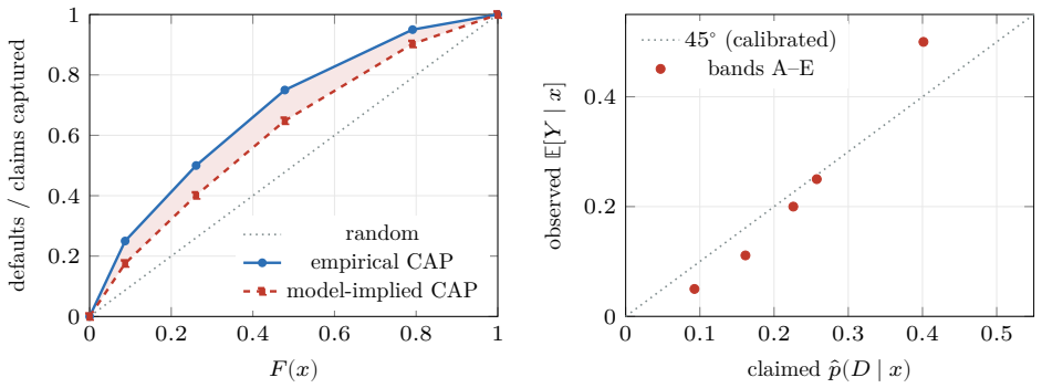
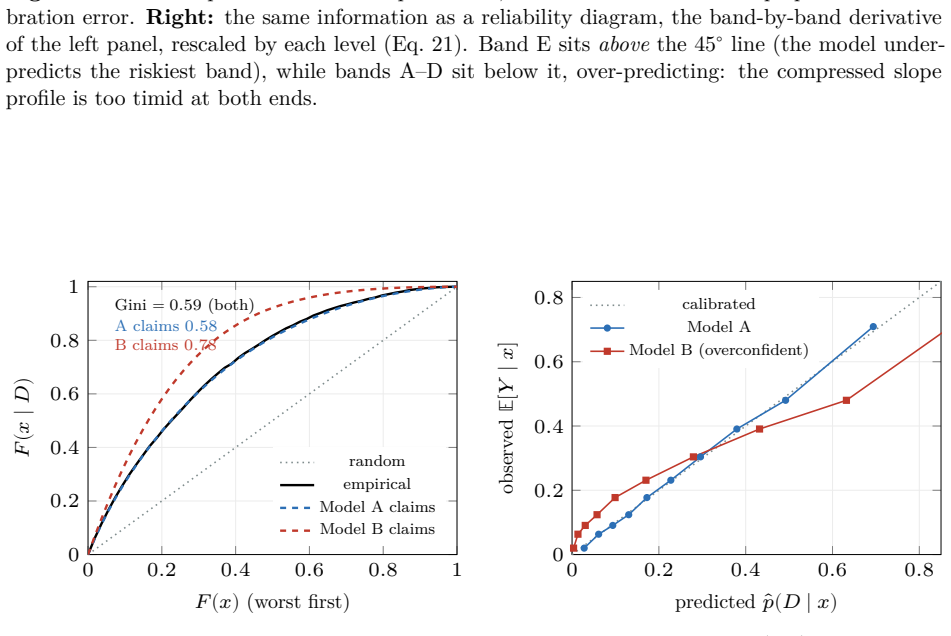
The CAP slope is Bayes' theorem in cumulative coordinates: the standardized PD it recovers is the posterior probability rescaled by the prior. The odds form places the weight of evidence inside one geometry with the information value. The accuracy ratio, Somers' D_xy, and the Gini (2A-1)/(1-p_D) are revealed as one number computed three ways. In comparison mode the identity recovers the reliability diagram in cumulative coordinates, with the sign of the gap between empirical and model-implied Gini coefficients serving as a calibration diagnostic.
What carries the argument
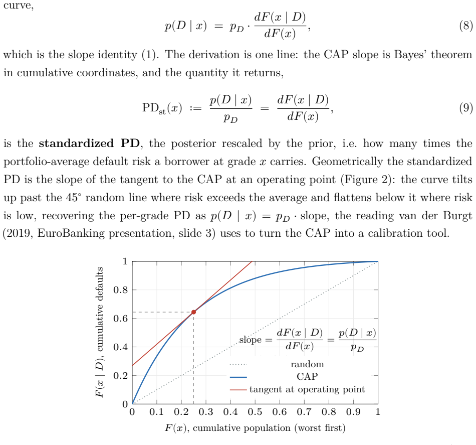
The CAP slope (dy/dx), identified as the likelihood ratio that converts prior default probability into posterior via the continuous identity p(D|x) = p_D dy/dx.
If this is right
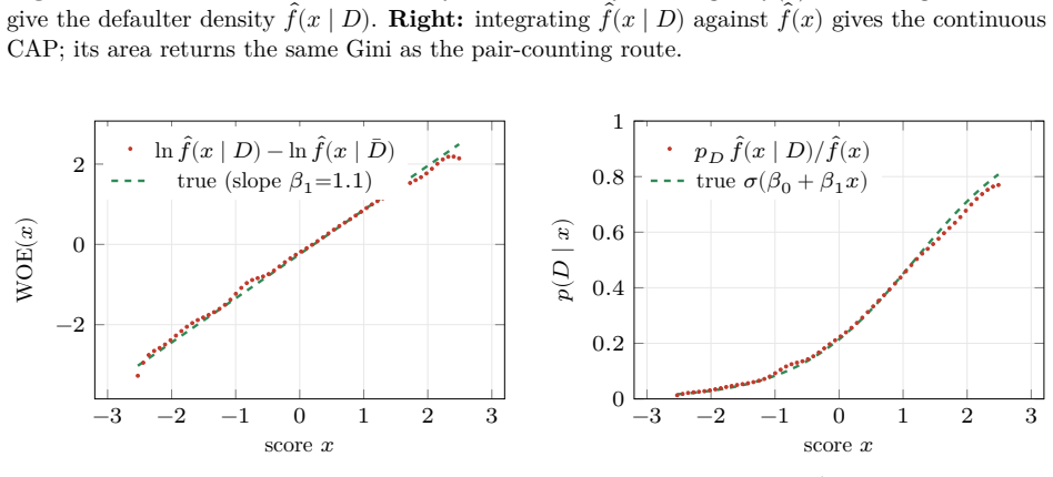
- Weight of evidence at each point equals the log of the ratio of the bad and good CAP slopes.
- Accuracy ratio, Somers' D, and Gini coefficient become interchangeable calculations of the same quantity.
- Comparison of model-implied and empirical Gini coefficients yields a signed calibration diagnostic in cumulative coordinates.
- The same geometry embeds the information value without separate likelihood computations.
Where Pith is reading between the lines
- The unification may let practitioners compute multiple discrimination and calibration metrics from a single CAP plot rather than separate tables.
- The cumulative-coordinate view could extend naturally to time-to-event models by replacing the binary default indicator with a cumulative hazard.
- Kernel-density versions of the slope might provide nonparametric confidence bands around the recovered posterior without parametric assumptions on the score distribution.
Load-bearing premise
The continuous identity relating local default probability to prior times CAP slope is taken as already established rather than re-derived.
What would settle it
Compute the posterior default probability directly from Bayes' theorem on a scored dataset and compare it to the value recovered from the CAP slope at the same percentile; any systematic mismatch would falsify the identification.
Figures
read the original abstract
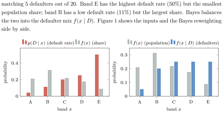
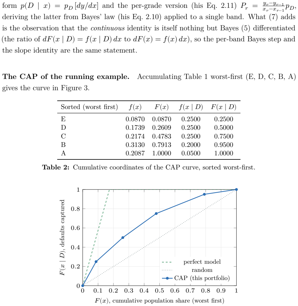
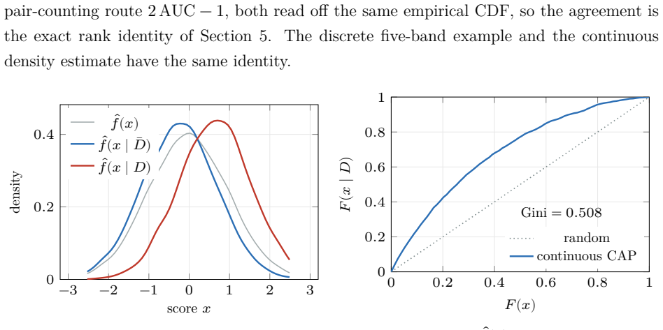
The probabilistic reading of the cumulative accuracy profile (CAP) has a long industry lineage. Falkenstein, Boral and Carty (2000) state, in discrete form, that the default rate at a score percentile equals the portfolio average rate times the local slope of the power curve; van der Burgt (2008, 2019) formalizes this as the continuous identity $p(D\mid x) = p_D\, dy/dx$ and imports the continuous form as a working fact; Tasche (2009) analyzes the resulting calibration method; Voloshyn and Voloshyn (2023) substitute Bayes' theorem, $f(x\mid D)=p(D\mid x) f(x)/p_D$, into the area integral and write the Gini as a functional of the calibration curve. The slope itself is already in the lineage (van der Burgt's $dy/dx$ is the ratio of the two cumulative differentials), but it enters as a cited working fact, never as Bayes' theorem. We make that identification explicit and draw out its consequences. First, the CAP slope is Bayes' theorem in cumulative coordinates: the standardized PD it recovers is the posterior probability rescaled by the prior. The weight of the paper then falls on two results this reading unlocks. The odds form places the weight of evidence (the log of the likelihood ratio, i.e. the Bayes factor) and the information value inside one geometry (the weight of evidence at a point is the log of the ratio of the "bad" and "good" CAP slopes). The accuracy ratio, Somers' $D_{xy}$, and the Gini $(2A-1)/(1-p_D)$ are revealed as one number computed three ways. Run in comparison mode (realized outcomes against model claims), the same identity recovers the reliability diagram in cumulative coordinates, with the sign of the gap between the empirical and model-implied Gini coefficients as a calibration diagnostic. A worked five-band example carries every identity in discrete form, and a kernel-density example extends them to the continuous case.
Editorial analysis
A structured set of objections, weighed in public.
Referee Report
Summary. The manuscript identifies the slope of the cumulative accuracy profile (CAP) dy/dx with the rescaled posterior p(D|x)/p_D, framing this as Bayes' theorem in cumulative coordinates. It shows that this yields the weight of evidence as the log-ratio of bad and good CAP slopes, unifies the accuracy ratio, Somers' D, and Gini coefficient (via (2A-1)/(1-p_D)) as equivalent scalars, and recovers a cumulative reliability diagram whose gap between empirical and model-implied Gini serves as a calibration diagnostic. The claims are instantiated in a five-band discrete example and a kernel-density continuous case, building on prior work by van der Burgt, Tasche, and Voloshyn.
Significance. If the identification holds, the result supplies a parameter-free geometric-probabilistic unification of several standard credit-risk quantities (CAP slope, WoE/IV, AR/Somers' D/Gini, cumulative calibration) whose algebraic consequences follow directly from the CAP definition and the fundamental theorem of calculus. The explicit Bayes reading had remained implicit in the cited lineage; surfacing it may improve interpretability and diagnostic practice without new assumptions or fitted parameters.
minor comments (3)
- [continuous example] § on the continuous case: the kernel-density example should explicitly state whether the bandwidth choice affects the recovered posterior or only the visual smoothness, to confirm invariance of the slope-Bayes identity.
- [discrete example] The five-band discrete table would benefit from an additional column showing the explicit likelihood ratio at each band to make the WoE-as-log-slope-ratio identity immediately verifiable by the reader.
- [calibration section] Notation: distinguish the model-implied CAP from the empirical CAP more consistently when discussing the reliability-diagram gap; the current text occasionally uses the same symbol for both.
Simulated Author's Rebuttal
We thank the referee for the accurate summary of the manuscript and the positive assessment of its significance. The recommendation for minor revision is noted. No specific major comments were provided in the report.
Circularity Check
No significant circularity identified
full rationale
The paper imports the identity p(D|x) = p_D dy/dx from the external citation van der Burgt (2008, 2019) as a working fact and then equates the slope to the Bayes factor form p(x|D)/p(x). This equivalence follows immediately from the CAP definition y(x) = p_D^{-1} ∫_0^x p(D|t) dt by the fundamental theorem of calculus, with no fitted parameters, self-referential definitions, or load-bearing self-citations required. All downstream claims (WoE as log-ratio of bad/good slopes, AR = Somers' D = Gini/(1-p_D), calibration diagnostics) are direct algebraic rewritings of the same identity. No quoted step reduces to its inputs by construction, and the derivation remains self-contained against external benchmarks.
Axiom & Free-Parameter Ledger
axioms (2)
- standard math Bayes' theorem relating posterior, likelihood and prior
- domain assumption Continuous identity p(D|x) = p_D dy/dx from van der Burgt (2008, 2019)
Reference graph
Works this paper leans on
-
[1]
Alvarez-Melis, D., Jaakkola, T., and Jegelka, S. (2019). Weight of Evidence as a Basis for Human-Oriented Explanations . arXiv:1910.13503
arXiv 2019
-
[2]
Alvarez-Melis, D., Kaur, H., Daumé III, H., Wallach, H., and Wortman Vaughan, J. (2021). From Human Explanation to Model Interpretability: A Framework Based on Weight of Evidence . arXiv:2104.13299
arXiv 2021
-
[3]
Falkenstein, E., Boral, A., and Carty, L. V. (2000). RiskCalc for Private Companies: Moody’s Default Model. Rating Methodology, Global Credit Research, Moody’s Investors Service
2000
-
[4]
Good, I. J. (1950). Probability and the Weighing of Evidence . Charles Griffin, London
1950
-
[5]
Good, I. J. (1985). Weight of evidence: a brief survey. In J. M. Bernardo, M. H. DeGroot, D. V. Lindley, and A. F. M. Smith (eds.), Bayesian Statistics 2 , pp. 249–270. North- Holland
1985
-
[6]
Guo, C., Pleiss, G., Sun, Y., and Weinberger, K. Q. (2017). On calibration of mod- ern neural networks. In Proceedings of the 34th International Conference on Machine Learning (ICML), pp. 1321–1330
2017
-
[7]
nonparametric
Newson, R. (2002). Parameters behind “nonparametric” statistics: Kendall’s 𝜏 , Somers’ 𝐷 and median differences. The Stata Journal 2(1), 45–64. 18
2002
-
[8]
Somers, R. H. (1962). A new asymmetric measure of association for ordinal variables. American Sociological Review 27(6), 799–811
1962
-
[9]
Sudjianto, A., and Burakov, D. (2025). An Information-Theoretic Framework for Credit Risk Modeling: Unifying Industry Practice with Statistical Theory for Fair and Inter- pretable Scorecards. arXiv:2509.09855
arXiv 2025
-
[10]
Tasche, D. (2005). Rating and probability of default validation. Working Paper 14, Studies on the Validation of Internal Rating Systems, Basel Committee on Banking Supervision, Bank for International Settlements
2005
-
[11]
Tasche, D. (2009). Estimating Discriminatory Power and PD Curves When the Number of Defaults Is Small . arXiv:0905.3928
Pith/arXiv arXiv 2009
-
[12]
Thomas, L. C. (2009). Consumer Credit Models: Pricing, Profit and Portfolios . Oxford University Press
2009
-
[13]
van der Burgt, M. J. (2008). Calibrating low-default portfolios, using the cumulative accuracy profile. Journal of Risk Model Validation 1(4), 17–33
2008
-
[14]
van der Burgt, M. J. (2019). Calibration and mapping of credit scores by riding the cumulative accuracy profile. Journal of Credit Risk 15(1), 1–25. https://doi.org/10. 21314/JCR.2018.240
2019
-
[15]
CAP as calibration tool
van der Burgt, M. J. (2019). Calibration and Mapping of Credit Scores by Riding the Cumulative Accuracy Profile . Presentation, EuroBanking 2019, Ljubljana, 26–29 May (slide 3, “CAP as calibration tool”)
2019
-
[16]
Voloshyn, M., and Voloshyn, I. (2023). On Factors Affecting the Change in the Gini Coefficient of the Credit Scoring Model . ScienceOpen Preprint. https://doi.org/10. 14293/PR2199.000388.v1. 19
arXiv 2023
discussion (0)
Sign in with ORCID, Apple, or X to comment. Anyone can read and Pith papers without signing in.