Hierarchical separation of relaxation timescales from spectral localization bounds
Pith reviewed 2026-06-26 16:42 UTC · model grok-4.3
The pith
Strong system-bath coupling produces a hierarchy of population relaxation timescales via bright-dark mode structure in the generalized V model.
A machine-rendered reading of the paper's core claim, the machinery that carries it, and where it could break.
Core claim
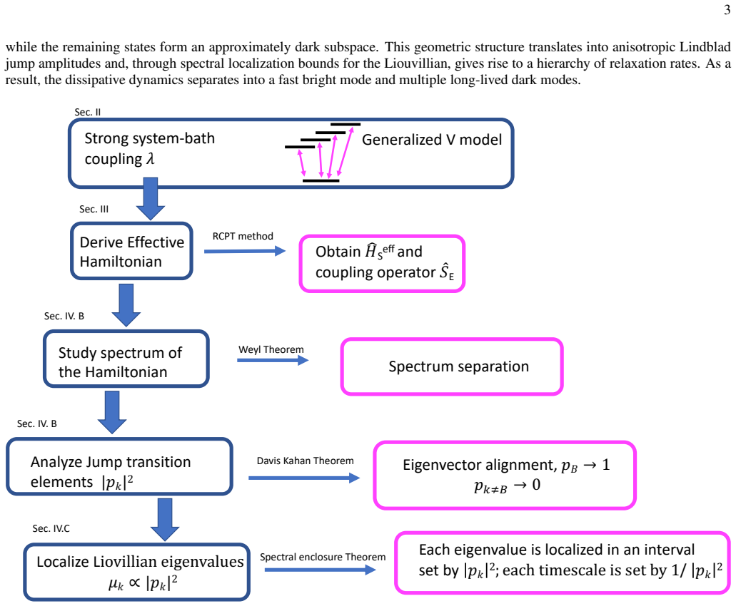
For the generalized V model, strong system-bath coupling gives rise to a bright-dark structure in the effective system-bath coupling operator: a single collective mode remains strongly coupled to the environment, while the remaining modes become progressively dark. Consequently, the dynamics separate into fast and slow sectors and, at finite coupling strengths, develop a hierarchy of population relaxation timescales.
What carries the argument
Reaction-coordinate polaron transform that maps the strong-coupling problem onto an effective weakly dissipative model, combined with spectral localization bounds on the spectrum of the resulting Liouvillian superoperator.
If this is right
- Dynamics separate into fast and slow sectors.
- A hierarchy of population relaxation timescales develops at finite coupling strengths.
- Dissipative dynamics exhibit pronounced slowing down at strong coupling.
- Long-lived states can be engineered through system-environment interactions.
- Both secular and non-secular quantum master equations corroborate the timescale separation.
Where Pith is reading between the lines
- The bright-dark mechanism may apply to other multilevel open quantum systems beyond the specific V model considered.
- Localization bounds could allow analytical estimates of relaxation rates without full numerical diagonalization of the Liouvillian.
- The separation might be harnessed in quantum devices to protect selected states from rapid environmental decay.
- Similar hierarchical relaxation could appear in other strong-coupling platforms such as circuit QED or molecular systems.
Load-bearing premise
The reaction-coordinate polaron transform produces an effective Liouvillian whose spectrum can be bounded by localization arguments that remain valid at finite coupling and whose eigenmode structure directly controls the population relaxation rates extracted from the master equation.
What would settle it
Numerical simulations of the generalized V model at strong but finite coupling that show no separation into distinct fast and slow population relaxation timescales would falsify the claim.
Figures


read the original abstract
We investigate the dissipative dynamics of multilevel quantum systems strongly coupled either to a lossy cavity mode or directly to a bosonic environment. By deriving spectral localization bounds, we establish conditions under which strong system-bath coupling gives rise to a hierarchy of population relaxation timescales. Our approach builds on the reaction-coordinate polaron-transform framework. By mapping the original strong-coupling problem onto an effective weakly dissipative model, we analyze the spectrum of the resulting Liouvillian superoperator through localization bounds. For the generalized V model, we find that strong system-bath coupling gives rise to a bright-dark structure in the effective system-bath coupling operator: a single collective mode remains strongly coupled to the environment, while the remaining modes become progressively dark. Consequently, the dynamics separate into fast and slow sectors and, at finite coupling strengths, develop a hierarchy of population relaxation timescales. Numerical simulations based on both secular and non-secular quantum master equations corroborate the emergence of timescale separation and the pronounced slowing down of dissipative dynamics at strong coupling. Our results reveal a general mechanism underlying anomalously slow relaxation in strongly coupled open quantum systems and provide a route for engineering long-lived states through system-environment interactions.
Editorial analysis
A structured set of objections, weighed in public.
Referee Report
Summary. The paper claims that reaction-coordinate polaron transforms map strongly coupled open quantum systems to effective weakly dissipative models whose Liouvillian spectra obey localization bounds. These bounds imply a bright-dark structure in the effective system-bath coupling for the generalized V model (one collective mode remains bright while others become progressively dark), producing a hierarchy of population relaxation timescales at finite coupling. Secular and non-secular master-equation simulations are said to corroborate the timescale separation.
Significance. If the localization bounds hold with controlled error at finite residual coupling and directly govern the extracted relaxation rates, the result supplies a general, non-perturbative mechanism for anomalously slow dissipation and a route to engineer long-lived states via system-environment coupling. The combination of polaron mapping with spectral localization arguments is a distinctive technical contribution.
major comments (2)
- [Derivation of spectral localization bounds and effective Liouvillian] The central claim requires that the localization bounds on the effective Liouvillian remain valid and control population relaxation rates at finite (not asymptotically weak) residual coupling after the polaron transform. The manuscript provides no explicit error estimates, regime-of-validity proof, or demonstration that standard localization arguments extend beyond perturbative or infinite-system limits when dissipation is only moderately weak; this directly affects whether the bright-dark eigenmode structure determines the observed timescale hierarchy for the generalized V model.
- [Polaron-transform framework and effective model construction] The reaction-coordinate polaron mapping is asserted to produce an effective model whose spectrum yields the claimed hierarchy without hidden parameter dependence, yet no quantitative bound is given on the approximation error introduced by the transform or by any truncation in the effective bath. Without this, it is unclear whether the separation into fast and slow sectors survives at the finite coupling strengths used in the simulations.
minor comments (1)
- [Numerical simulations] Clarify in the simulation section whether any post-hoc truncation or choice of reaction-coordinate parameters was made after inspecting the data, and state explicitly how this choice was shown not to affect the reported timescale hierarchy.
Simulated Author's Rebuttal
We thank the referee for their thorough review and constructive comments. The concerns regarding the validity of the localization bounds and the polaron mapping at finite coupling are well taken, and we respond to each point below.
read point-by-point responses
-
Referee: The central claim requires that the localization bounds on the effective Liouvillian remain valid and control population relaxation rates at finite (not asymptotically weak) residual coupling after the polaron transform. The manuscript provides no explicit error estimates, regime-of-validity proof, or demonstration that standard localization arguments extend beyond perturbative or infinite-system limits when dissipation is only moderately weak; this directly affects whether the bright-dark eigenmode structure determines the observed timescale hierarchy for the generalized V model.
Authors: The spectral localization bounds are derived in Section III by applying operator localization techniques to the effective Liouvillian obtained after the reaction-coordinate polaron transform. These bounds are formulated directly in terms of the residual coupling strength and do not rely on a perturbative expansion in that strength. Their implications for the bright-dark structure in the generalized V model are then verified by the secular and non-secular master-equation simulations performed at finite coupling (Section IV). We agree that an explicit discussion of the regime of validity would strengthen the presentation and will add a dedicated paragraph outlining the conditions under which the bounds remain controlling. revision: yes
-
Referee: The reaction-coordinate polaron mapping is asserted to produce an effective model whose spectrum yields the claimed hierarchy without hidden parameter dependence, yet no quantitative bound is given on the approximation error introduced by the transform or by any truncation in the effective bath. Without this, it is unclear whether the separation into fast and slow sectors survives at the finite coupling strengths used in the simulations.
Authors: The reaction-coordinate polaron transform is an exact unitary mapping that shifts the strong-coupling interaction into a displaced bath; the resulting residual system-bath coupling is controlled by the reaction-coordinate frequency, which is chosen to minimize its norm. The effective bath truncation is likewise controlled by this choice, as described in the methods. We concur that an explicit quantitative estimate of the residual error at the coupling strengths used in the numerics would be useful and will include such a bound (based on the operator norm of the residual interaction) in the revised manuscript. revision: yes
Circularity Check
No circularity; derivation applies external mapping and bounds without reduction to inputs
full rationale
The provided abstract and description show the paper mapping the strong-coupling problem via the reaction-coordinate polaron transform to an effective model, then applying spectral localization bounds to identify bright-dark structure and timescale hierarchy in the generalized V model. No quoted equations or steps reduce a claimed prediction or result to a fitted parameter, self-definition, or load-bearing self-citation chain. The central claim is presented as following from the spectrum analysis of the mapped Liouvillian, which is treated as independent of the target hierarchy. Concerns about bound validity at finite coupling are correctness issues, not circularity. The derivation is self-contained against the stated framework.
Axiom & Free-Parameter Ledger
axioms (2)
- domain assumption The reaction-coordinate polaron transform yields an effective Liouvillian whose spectrum controls population relaxation rates.
- domain assumption Spectral localization bounds can be derived for the transformed Liouvillian and remain informative at finite coupling.
Reference graph
Works this paper leans on
-
[1]
(9) we treat the spectrum ofˆHeff S (λ,Ω)perturbatively
Properties of the effective Hamiltonian Going back to the effective system Hamiltonian in Eq. (9) we treat the spectrum ofˆHeff S (λ,Ω)perturbatively. First, we rewrite it as ˆHeff S (λ,Ω)=D 1⊕ˆM(λ,Ω).(16) Here,D 1 is the1×1top-left decoupled block and ˆM(λ,Ω)is the bottom-right(N−1)×(N−1)block in Eq. (9). Let us focus on ˆM(λ,Ω), re-expressing it as ˆM= ...
-
[2]
Consequently, one eigenstate aligns with the coupling vector while all others become orthogonal to it, producing dark states
Strong coupling generates a rank-one bright projector in the effective Hamiltonian. Consequently, one eigenstate aligns with the coupling vector while all others become orthogonal to it, producing dark states. As we discuss next, this property translates to the occurrence of one bright (fast) mode andN−2dark (diverging timescales) modes in the dissipative...
-
[3]
(11) are suppressed in this limit
Properties of the Liouvillian Since all but one of the projection amplitudes diminish at the ultrastrong coupling limit, all but one of the Lindblad jump operators in Eq. (11) are suppressed in this limit. Physically, this represents a scenario in which only a single bath-induced jump process remains active in the energy eigenbasis of ˆHeff S , while all ...
-
[4]
The spectrum of the corresponding effective Hamiltonian is shown in Fig. 5(a). Inverse squared projection amplitudes are presented in Fig. 5(b). At weak coupling, the system coupling operator connects the ground state to all excited states with the same amplitude. Strong system-bath coupling generates a pronounced anisotropy in the effective transition am...
-
[5]
bright” mode remains strongly coupled to the bath and relaxes rapidly, while the remaining “dark
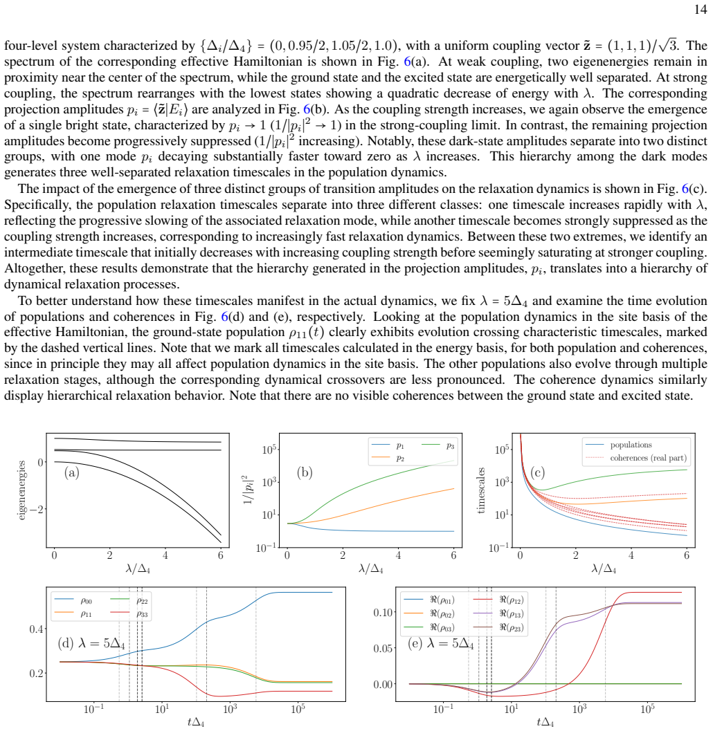
The spectrum of the corresponding effective Hamiltonian is shown in Fig. 6(a). At weak coupling, two eigenenergies remain in proximity near the center of the spectrum, while the ground state and the excited state are energetically well separated. At strong coupling, the spectrum rearranges with the lowest states showing a quadratic decrease of energy with...
-
[6]
(6) for the Generalized V model Hamiltonian coupled to a bosonic bath
Derivation of the effective GVM Hamiltonian Here, we derive the effective Hamiltonian ˆHeff S (λ,Ω)using Eq. (6) for the Generalized V model Hamiltonian coupled to a bosonic bath. In the RCPT procedure, we first need to apply the polaron transform onto the originalN-level system. We 18 introduce the following notation for the polaron unitary, ˆUP =exp[ λ ...
-
[7]
Example: Standard V Model We exemplify the form of the effective Hamiltonian on theVmodel withN=3in Eq. (1). TheVmodel system’s Hamiltonian is ˆHS = ⎛ ⎜ ⎝ 0 0 0 0 ∆ 2 0 0 0 ∆ 3 ⎞ ⎟ ⎠ .(A14) The coupling matrix allows transitions from the ground state to each excited state, ˜z† =(1,1)/ √ 2, ˆS= 1√ 2 ⎛ ⎜ ⎝ 0 1 1 1 0 0 1 0 0 ⎞ ⎟ ⎠ ,(A15) From Eq. (9) we obta...
-
[8]
Decomposition of the effective Hamiltonian into bright and dark state subspaces We define bright and dark projectors as ˆb=˜ z˜ z†, ˆd= ˆIN−1−ˆb, i.e., ˆbprojects onto the coupling vector˜ z, which accounts for bath-system interactions, and ˆdis the complement projection. Then ˆM(λ,Ω)= ˆ∆+(e −λ2/(2Ω2)−1)(ˆb ˆ∆+ ˆ∆ˆb)+ ⎡⎢⎢⎢⎣ 1+e −2λ2/Ω2 2 −2e−λ2/(2Ω2)+1 ⎤⎥...
-
[9]
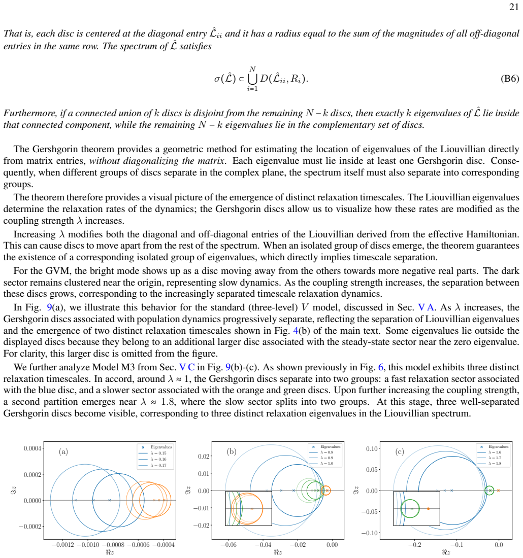
(b)-(c) Discs for a four-level GVM of Fig. 6. The chosen values ofλindicate on two stages of timescale separation. Appendix C: Relaxation Timescales at Finite Strong Coupling We prove here that a hierarchal structure ofpk =⟨˜z∣Ek⟩shows as a separation of relaxation timescales at finiteλ. Specifically, we argue that for a wide range ofλ, the population rel...
-
[10]
Proof for a general localization of eigenvalues,µ k ∈(−αk+1,−αk) To begin, we recast Eq. (26) as ˆL=−ˆD−β1T , β∶= ⎛ ⎜⎜⎜ ⎝ β2 β3 ⋮ βN ⎞ ⎟⎟⎟ ⎠ ,1∶= ⎛ ⎜⎜⎜ ⎝ 1 1 ⋮ 1 ⎞ ⎟⎟⎟ ⎠ , ˆD=diag(α i)i>1 .(C1) Using the matrix determinant lemma, det( ˆA+uv T)=det( ˆA)(1+v T ˆA−1u) ,(C2) with ˆA=−( ˆD+µ ˆI),u=β, andv=1, the characteristic polynomial becomes det( ˆL−µˆI)= ...
-
[11]
While Eq
Refined interval,µ k ∈(−αk−kβk,−αk) Let us work in the same ordering convention, whereα 1 <α 2 <...<α N ;β 1 <β 2 <...<β N . While Eq. (C5) implies that µk ∈(−αk+1,−αk), we now seek the sharper localizationµ k ∈(−αk −kβk,−αk). To establish this refinement, we impose a separation condition on the decay rates,α k+1−αk ≥∑i≤kβi. Physically, this condition sta...
-
[12]
Bounding eigenvalues with averaged dark state transition frequencies To obtain a more transparent expression for the Liouvillian eigenvalues, we approximate the dark-state transition frequencies by their average value, ¯E= 1 N−2∑k≠1,BEk1. We now show that for sufficiently strong coupling, the dark-state transition frequencies cluster around ¯E, and theref...
-
[13]
Bound on the gap between adjacent eigenvalues Since each Liouvillian eigenvalue scales proportionally to∣pk∣2, it implies that ∣µk∣≍λ ∣pk∣2, τ k =−1 µk ≍λ 1 ∣pk∣2 .(C25) x≍λ ymeans that there existsλdependent factorsC 1(λ), C2(λ)such thatC 1(λ)y≤x≤C 2(λ)y∀λ∈R+. Furthermore, comparing the localization intervals forµ k andµ k+1, we obtain the lower bound ∣µ...
-
[14]
M. Stefanini, A. A. Ziolkowska, D. Budker, U. Poschinger, F. Schmidt-Kaler, A. Browaeys, A. Imamoglu, D. Chang, and J. Marino, “Is lindblad for me?” (2026), arXiv:2506.22436 [quant-ph]
work page internal anchor Pith review Pith/arXiv arXiv 2026
-
[15]
Breuer and F
H.-P. Breuer and F. Petruccione,The Theory of Open Quantum Systems(Oxford University Press, 2007)
2007
-
[16]
Nitzan,Chemical Dynamics in Condensed Phases: Relaxation, Transfer, and Reactions in Condensed Molecular Systems, Oxford Graduate Texts (OUP Oxford, 2013)
A. Nitzan,Chemical Dynamics in Condensed Phases: Relaxation, Transfer, and Reactions in Condensed Molecular Systems, Oxford Graduate Texts (OUP Oxford, 2013)
2013
-
[17]
P. P. Hofer, M. Perarnau-Llobet, L. D. M. Miranda, G. Haack, R. Silva, J. B. Brask, and N. Brunner, New Journal of Physics19, 123037 (2017)
2017
-
[18]
Ashida, Z
Y . Ashida, Z. Gong, and M. Ueda, Advances in Physics69, 249 (2020). 26
2020
-
[19]
Quantum non-markovian hatano-nelson model,
S. K. Jana, R. Hanai, T. V . Vu, H. Hayakawa, and A. Purkayastha, “Quantum non-markovian hatano-nelson model,” (2025), arXiv:2511.05328 [quant-ph]
-
[20]
Denisov, T
S. Denisov, T. Laptyeva, W. Tarnowski, D. Chru´sci´nski, and K. ˙Zyczkowski, Phys. Rev. Lett.123, 140403 (2019)
2019
-
[21]
S. H. Tekur, M. S. Santhanam, B. K. Agarwalla, and M. Kulkarni, Phys. Rev. B110, L241410 (2024)
2024
-
[22]
Popkov, C
V . Popkov, C. Presilla, and M. Salerno, Phys. Rev. A111, L050202 (2025)
2025
-
[23]
Kopciuch and A
M. Kopciuch and A. Miranowicz, Phys. Rev. Res.7, 033187 (2025)
2025
-
[24]
Gaidash, A
A. Gaidash, A. D. Kiselev, A. Kozubov, and G. Miroshnichenko, Phys. Rev. A111, 062211 (2025)
2025
-
[25]
Akemann, M
G. Akemann, M. Kieburg, A. Mielke, and T. c. v. Prosen, Phys. Rev. Lett.123, 254101 (2019)
2019
-
[26]
L. S ´a, P. Ribeiro, and T. c. v. Prosen, Phys. Rev. X10, 021019 (2020)
2020
-
[27]
´Alvaro Rubio-Garc´ıa, R. A. Molina, and J. Dukelsky, SciPost Phys. Core5, 026 (2022)
2022
-
[28]
Prasad, H
M. Prasad, H. K. Yadalam, C. Aron, and M. Kulkarni, Phys. Rev. A105, L050201 (2022)
2022
-
[29]
Mori, Phys
T. Mori, Phys. Rev. B109, 064311 (2024)
2024
-
[30]
Can, Journal of Physics A: Mathematical and Theoretical52, 485302 (2019)
T. Can, Journal of Physics A: Mathematical and Theoretical52, 485302 (2019)
2019
-
[31]
Haga, Phys
T. Haga, Phys. Rev. B110, 104303 (2024)
2024
-
[32]
Akemann, F
G. Akemann, F. Balducci, A. Chenu, P. P¨aßler, F. Roccati, and R. Shir, Phys. Rev. Res.7, 013098 (2025)
2025
-
[33]
Barad, Q
R. Barad, Q. Tang, and X. Wen, Phys. Rev. B112, 235143 (2025)
2025
-
[34]
Wu and A
L.-N. Wu and A. Eckardt, Phys. Rev. B101, 220302 (2020)
2020
-
[35]
Minganti, A
F. Minganti, A. Biella, N. Bartolo, and C. Ciuti, Phys. Rev. A98, 042118 (2018)
2018
-
[36]
Fitzpatrick, N
M. Fitzpatrick, N. M. Sundaresan, A. C. Y . Li, J. Koch, and A. A. Houck, Phys. Rev. X7, 011016 (2017)
2017
-
[37]
Yuan, H.-R
D. Yuan, H.-R. Wang, Z. Wang, and D.-L. Deng, Phys. Rev. Lett.126, 160401 (2021)
2021
-
[38]
Wang and R
P. Wang and R. Fazio, Phys. Rev. A103, 013306 (2021)
2021
-
[39]
J. L. Li, D. C. Rose, J. P. Garrahan, and D. J. Luitz, Phys. Rev. B105, L180201 (2022)
2022
-
[40]
T. Can, V . Oganesyan, D. Orgad, and S. Gopalakrishnan, Phys. Rev. Lett.123, 234103 (2019)
2019
-
[41]
Y .-N. Zhou, L. Mao, and H. Zhai, Phys. Rev. Res.3, 043060 (2021)
2021
-
[42]
L. S ´a, P. Ribeiro, and T. Prosen, Journal of Physics A: Mathematical and Theoretical53, 305303 (2020)
2020
-
[43]
Costa, P
J. Costa, P. Ribeiro, A. D. Luca, T. Prosen, and L. S ´a, SciPost Phys.15, 145 (2023)
2023
-
[44]
Popkov and C
V . Popkov and C. Presilla, Phys. Rev. Lett.126, 190402 (2021)
2021
-
[45]
B. Min, M. Gerry, and D. Segal, Phys. Rev. A112, 062226 (2025)
2025
-
[46]
K. Wang, F. Piazza, and D. J. Luitz, Phys. Rev. Lett.124, 100604 (2020)
2020
-
[47]
N. D. Hartmann, J. L. Li, and D. J. Luitz, Phys. Rev. B109, 054203 (2024)
2024
-
[48]
Orgad, V
D. Orgad, V . Oganesyan, and S. Gopalakrishnan, Phys. Rev. Lett.132, 040403 (2024)
2024
-
[49]
O. E. Sommer, F. Piazza, and D. J. Luitz, Phys. Rev. Res.3, 023190 (2021)
2021
-
[50]
T. Haga, M. Nakagawa, R. Hamazaki, and M. Ueda, Phys. Rev. Res.5, 043225 (2023)
2023
-
[51]
T. V . Tscherbul and P. Brumer, Phys. Rev. Lett.113, 113601 (2014)
2014
-
[52]
T. V . Tscherbul and P. Brumer, The Journal of Chemical Physics142, 104107 (2015)
2015
-
[53]
Dodin and P
A. Dodin and P. Brumer, Journal of Physics B: Atomic, Molecular and Optical Physics54, 223001 (2021)
2021
-
[54]
Ivander, N
F. Ivander, N. Anto-Sztrikacs, and D. Segal, Phys. Rev. E108, 014130 (2023)
2023
-
[55]
Gerry, M
M. Gerry, M. J. Kewming, and D. Segal, Phys. Rev. Res.6, 033106 (2024)
2024
-
[56]
On truncations of hierarchical equations of motion for finite-dimensional systems
V . Vadimov, arXiv preprint arXiv:2604.22568 (2026), 10.48550/arXiv.2604.22568
work page internal anchor Pith review Pith/arXiv arXiv doi:10.48550/arxiv.2604.22568 2026
-
[57]
Anto-Sztrikacs, A
N. Anto-Sztrikacs, A. Nazir, and D. Segal, PRX Quantum4, 020307 (2023)
2023
-
[58]
Scali, J
S. Scali, J. Anders, and L. A. Correa, Quantum5, 451 (2021)
2021
-
[59]
T. V . Tscherbul, Phys. Rev. A112, 012208 (2025)
2025
-
[60]
Anto-Sztrikacs, H
N. Anto-Sztrikacs, H. J. D. Miller, A. Nazir, and D. Segal, Phys. Rev. A109, L060201 (2024)
2024
-
[61]
A. S. Trushechkin, M. Merkli, J. D. Cresser, and J. Anders, A VS Quantum Science4, 012301 (2022)
2022
-
[62]
Anto-Sztrikacs, B
N. Anto-Sztrikacs, B. Min, M. Brenes, and D. Segal, Phys. Rev. B108, 115437 (2023)
2023
-
[63]
Reservoir-mediated spin entanglement in the mean-force Gibbs state
L. A. Williamson, W. McEniery, F. Cerisola, and J. Anders, “Reservoir-mediated spin entanglement in the mean-force gibbs state,” (2026), arXiv:2604.26562 [quant-ph]
work page internal anchor Pith review Pith/arXiv arXiv 2026
-
[64]
B. Min, N. Anto-Sztrikacs, M. Brenes, and D. Segal, Phys. Rev. Lett.132, 266701 (2024)
2024
-
[65]
B. Min, K. Agarwal, and D. Segal, Phys. Rev. B110, 125415 (2024)
2024
-
[66]
Garwoła and D
J. Garwoła and D. Segal, Phys. Rev. B110, 174304 (2024)
2024
-
[67]
Garwoła and D
J. Garwoła and D. Segal, Phys. Rev. Res.8, L022039 (2026)
2026
-
[68]
L. A. Correa, B. Xu, B. Morris, and G. Adesso, The Journal of Chemical Physics151, 094107 (2019)
2019
-
[69]
Mahadeviya, S
K. Mahadeviya, S. V . Moreira, S. P. Mandal, M. Pandit, J. Prior, and M. T. Mitchison, New Journal of Physics28, 044511 (2026)
2026
-
[70]
G. D. Mahan,Many-Particle Physics, 3rd ed. (Kluwer Academic/Plenum Publishers, New York, 2000)
2000
-
[71]
Frisk Kockum, A
A. Frisk Kockum, A. Miranowicz, S. De Liberato, S. Savasta, and F. Nori, Nature Reviews Physics1, 19 (2019)
2019
-
[72]
Cavity-Induced Excitonic Insulation and Non-Fermi-Liquid Behavior in Dirac Materials
Y . Guo and Y . Ashida, “Cavity-induced excitonic insulation and non-fermi-liquid behavior in dirac materials,” (2026), arXiv:2605.10652 [cond-mat.str-el]
work page internal anchor Pith review Pith/arXiv arXiv 2026
-
[73]
Mochida and Y
J. Mochida and Y . Ashida, Phys. Rev. B110, 035158 (2024)
2024
-
[74]
Masuki and Y
K. Masuki and Y . Ashida, Phys. Rev. B109, 195173 (2024)
2024
-
[75]
Ashida, A
Y . Ashida, A. m. c.˙Imamo˘glu, and E. Demler, Phys. Rev. Lett.130, 216901 (2023)
2023
-
[76]
Masuki and Y
K. Masuki and Y . Ashida, Phys. Rev. B107, 195104 (2023)
2023
-
[77]
Ashida, A
Y . Ashida, A. m. c.˙Imamo˘glu, and E. Demler, Phys. Rev. Lett.126, 153603 (2021)
2021
-
[78]
Galego, F
J. Galego, F. J. Garcia-Vidal, and J. Feist, Phys. Rev. X5, 041022 (2015)
2015
-
[79]
Mandal, M
A. Mandal, M. A. Taylor, B. M. Weight, E. R. Koessler, X. Li, and P. Huo, Chem. Rev.123, 9786 (2023). 27
2023
-
[80]
Herrera and F
F. Herrera and F. C. Spano, Phys. Rev. Lett.116, 238301 (2016)
2016
discussion (0)
Sign in with ORCID, Apple, or X to comment. Anyone can read and Pith papers without signing in.