To select or not to select: predictively consistent priors instead of model selection
Pith reviewed 2026-06-26 07:50 UTC · model grok-4.3
The pith
Predictively consistent priors let complex models match or beat selected simpler ones in out-of-sample prediction.
A machine-rendered reading of the paper's core claim, the machinery that carries it, and where it could break.
Core claim
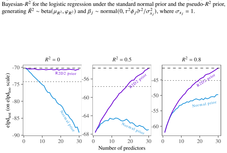
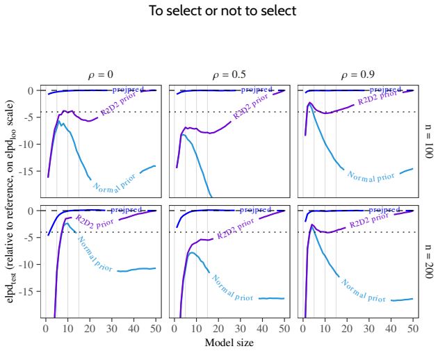
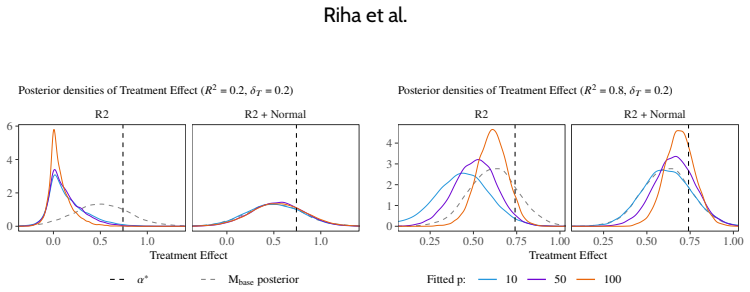
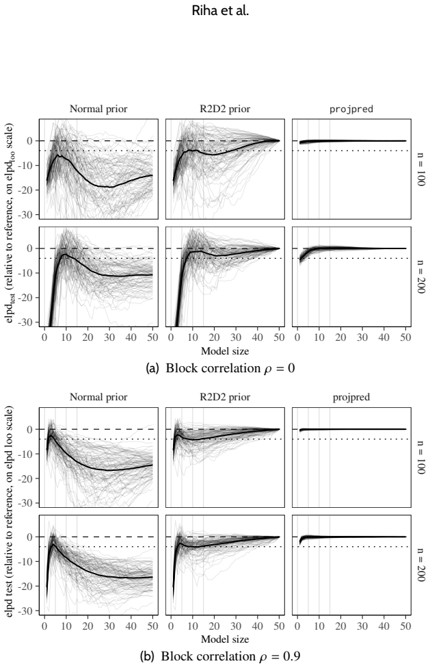
Predictively consistent priors keep prior predictive implications stable as model complexity increases. Flexible models equipped with such priors typically match or outperform selected simpler models in out-of-sample predictive performance across examples of adding covariates in linear and logistic regression, forward variable selection, and nonlinear modelling. When selection still improves performance, it signals that the original prior placed excessive mass on implausible predictive values. The authors therefore propose replacing sparsity or parsimony at the level of model components with the requirement that priors remain sensible in predictive space as models become more complex.
What carries the argument
Predictively consistent priors, defined as priors whose prior predictive distributions remain stable and sensible as model complexity increases.
If this is right
- Model selection can be omitted without harming predictive performance when priors satisfy the consistency condition.
- Cases where selection improves results point to prior predictive distributions that are already implausible before seeing data.
- Bayesian workflows can shift effort from comparing discrete models to designing priors that behave sensibly in predictive space.
- The same logic applies when adding covariates, performing variable selection, or moving to nonlinear structures.
Where Pith is reading between the lines
- Workflows that routinely fit one large model with such a prior may replace pipelines that enumerate and score many candidate models.
- The same prior-construction principle could be tested in settings beyond regression, such as time-series or spatial models where complexity also increases with added structure.
- If the stability condition proves hard to satisfy in some model classes, hybrid approaches that combine consistent priors with light selection might still be useful.
Load-bearing premise
Priors can be constructed so that their predictive implications stay stable and reasonable when model complexity grows.
What would settle it
A controlled experiment in which a flexible model with a predictively consistent prior is outperformed by a selected simpler model on out-of-sample predictive metrics across several independent datasets.
Figures


read the original abstract
Bayesian modelling workflows often consider multiple candidate models of varying complexity. Model selection is commonly used to navigate potential trade-offs between model complexity and generalisability to new data. We study when model selection is unnecessary or can even be harmful for predictive performance in finite data regimes and find that the need for selecting simpler models can depend on prior choice. We formalise predictively consistent priors, which keep prior predictive implications stable as model complexity increases. Across examples and numerical experiments, including adding covariates in linear and logistic regression, forward variable selection, and nonlinear modelling, flexible models with predictively consistent priors typically match or outperform selected simpler models in out-of-sample predictive performance. When selection helps, it can indicate poor joint prior implications, such as excessive prior mass on implausible predictive values. Based on our findings, we propose replacing the notion of sparsity or parsimony at the level of model components with specifying priors that remain sensible in predictive space as models become more complex.
Editorial analysis
A structured set of objections, weighed in public.
Referee Report
Summary. The paper claims that model selection can be unnecessary or harmful for out-of-sample predictive performance when using predictively consistent priors, which are priors designed to keep prior predictive distributions stable as model complexity increases (e.g., by adding covariates). Across linear and logistic regression, forward variable selection, and nonlinear modeling examples and numerical experiments, flexible models equipped with such priors typically match or outperform selected simpler models. The authors further claim that selection only improves performance when the joint prior is already misspecified in predictive space, and recommend replacing notions of sparsity with priors that remain sensible in predictive space as complexity grows.
Significance. If the central empirical claims hold under more detailed scrutiny, the work offers a substantive alternative perspective in Bayesian statistical methodology: shifting emphasis from post-hoc model selection to upfront prior specification that preserves predictive properties. The numerical demonstrations across multiple model classes provide concrete, falsifiable evidence that could influence prior elicitation practices and reduce reliance on selection procedures in finite-data regimes. The framing of predictively consistent priors as a generalizable concept (rather than ad-hoc per example) is a strength if the construction method generalizes beyond the reported cases.
major comments (2)
- [§4] §4 (numerical experiments): The central claim rests on out-of-sample performance comparisons, yet the manuscript provides insufficient detail on the exact predictive metrics employed (e.g., whether log predictive density, CRPS, or MSE), the precise construction rules for the predictively consistent priors in each setting, and any controls for data exclusion or cross-validation scheme. These omissions are load-bearing because they prevent assessment of whether the reported superiority is robust or sensitive to implementation choices.
- [Formalisation] Formalisation section: The definition of predictively consistent priors is presented primarily through examples rather than a general, model-class-independent construction that guarantees stability of the prior predictive as complexity increases; without this, the weakest assumption (that such priors exist and can be specified for arbitrary flexible models) remains demonstrated only case-by-case rather than established as a general principle.
minor comments (2)
- [Abstract] The abstract and introduction introduce the term 'predictively consistent priors' without an immediate formal definition or reference to the section where it is defined, which would improve readability for readers unfamiliar with the concept.
- [Formalisation] Notation for prior predictive distributions could be clarified with an explicit equation early in the formalisation to distinguish it from posterior predictive quantities.
Simulated Author's Rebuttal
We thank the referee for the detailed and constructive report. The comments highlight areas where additional clarity will strengthen the manuscript. We address each major comment below and indicate the revisions we will make.
read point-by-point responses
-
Referee: [§4] §4 (numerical experiments): The central claim rests on out-of-sample performance comparisons, yet the manuscript provides insufficient detail on the exact predictive metrics employed (e.g., whether log predictive density, CRPS, or MSE), the precise construction rules for the predictively consistent priors in each setting, and any controls for data exclusion or cross-validation scheme. These omissions are load-bearing because they prevent assessment of whether the reported superiority is robust or sensitive to implementation choices.
Authors: We agree that greater detail is needed for reproducibility. In the revision we will expand §4 to specify the predictive metrics (primarily log predictive density, with MSE and CRPS where used), the exact construction rules applied to obtain predictively consistent priors in each regression and nonlinear example, and the cross-validation scheme including data partitioning and any exclusion rules. revision: yes
-
Referee: [Formalisation] Formalisation section: The definition of predictively consistent priors is presented primarily through examples rather than a general, model-class-independent construction that guarantees stability of the prior predictive as complexity increases; without this, the weakest assumption (that such priors exist and can be specified for arbitrary flexible models) remains demonstrated only case-by-case rather than established as a general principle.
Authors: The formalisation section defines predictively consistent priors via the requirement that the prior predictive distribution remains stable (in a suitable sense) under increases in model complexity. While concrete constructions are illustrated case-by-case, the underlying principle is stated generally. We will revise the section to separate the general definition more clearly from the examples and to discuss the extent to which the principle can be applied to other model classes without providing a single algorithmic template that covers all cases. revision: partial
Circularity Check
No significant circularity detected
full rationale
The paper formalizes predictively consistent priors as a definition that stabilizes prior predictive distributions under increasing model complexity, then demonstrates via numerical experiments (linear/logistic regression, variable selection, nonlinear cases) that flexible models using these priors match or exceed the out-of-sample performance of selected simpler models. No load-bearing derivation, equation, or self-citation reduces the performance claims to fitted inputs or definitional equivalence; the argument is empirical and self-contained against external benchmarks. No steps meet the circularity criteria.
Axiom & Free-Parameter Ledger
axioms (2)
- domain assumption Bayesian modelling workflows often consider multiple candidate models of varying complexity
- domain assumption Model selection is commonly used to navigate potential trade-offs between model complexity and generalisability
invented entities (1)
-
predictively consistent priors
no independent evidence
Reference graph
Works this paper leans on
-
[1]
Vershynin, Roman , year =. High-
-
[2]
Mathematics of the USSR-Sbornik , author =
Distribution of eigenvalues for some sets of random matrices , volume =. Mathematics of the USSR-Sbornik , author =. 1967 , pages =
1967
-
[3]
, year =
Bai, Zhidong and Silverstein, Jack W. , year =. Spectral
-
[4]
Hahn, P. Richard and Murray, Jared S. and Carvalho, Carlos M. , month = sep, year =. Bayesian. Bayesian Analysis , publisher =. doi:10.1214/19-BA1195 , abstract =
-
[5]
Social Science & Medicine , author =
Understanding and misunderstanding randomized controlled trials , volume =. Social Science & Medicine , author =. 2018 , keywords =. doi:10.1016/j.socscimed.2017.12.005 , abstract =
-
[6]
Kuhn, Daniel and Esfahani, Peyman Mohajerin and Nguyen, Viet Anh and Shafieezadeh-Abadeh, Soroosh , month = oct, year =. Wasserstein. Operations. doi:10.1287/educ.2019.0198 , urldate =
-
[7]
Kohns, David and Kallioinen, Noa and McLatchie, Yann and Vehtari, Aki , month = jan, year =. The. Bayesian Analysis , publisher =. doi:10.1214/25-BA1512 , abstract =
-
[8]
Sharpening
Jefferys, William H and Berger, James O , year =. Sharpening
-
[9]
Journal of Economic Literature , author =
Potential. Journal of Economic Literature , author =. 2020 , keywords =. doi:10.1257/jel.20191597 , abstract =
-
[10]
Husain, Hisham , month = jun, year =. Distributional. 34th. doi:10.48550/arXiv.2006.04349 , abstract =
-
[11]
Hünermund, Paul and Louw, Beyers , month = jan, year =. On the. Organizational Research Methods , publisher =. doi:10.1177/10944281231219274 , abstract =
-
[12]
Ghojogh, Benyamin and Crowley, Mark , month = may, year =. The. doi:10.48550/arXiv.1905.12787 , abstract =
-
[13]
George, Edward I. , year =. The. Journal of the American Statistical Association , publisher =. doi:10.2307/2669776 , number =
-
[14]
The garden of forking paths:
Gelman, Andrew and Loken, Eric , year =. The garden of forking paths:
-
[15]
Geisser, Seymour and Eddy, William F. , year =. A. Journal of the American Statistical Association , publisher =. doi:10.2307/2286745 , abstract =
-
[16]
International Statistical Review , author =
Priors in. International Statistical Review , author =. 2022 , note =. doi:10.1111/insr.12502 , abstract =
-
[17]
On the marginal likelihood and cross-validation , volume =. Biometrika , author =. 2020 , pages =. doi:10.1093/biomet/asz077 , abstract =
-
[18]
Flam-Shepherd, Daniel and Requeima, James and Duvenaud, David , month = jan, year =. Mapping. 31st
-
[19]
Characterizing and
Flam-Shepherd, Daniel and Requeima, James and Duvenaud, David , pages =. Characterizing and. Third workshop on
-
[20]
free range statistics , author =
Stepwise selection of variables in regression is. free range statistics , author =. 2024 , note =
2024
-
[21]
How to select predictive models for decision-making or causal inference , volume =. GigaScience , author =. 2025 , pages =. doi:10.1093/gigascience/giaf016 , abstract =
-
[22]
Dawid, A. P. and Stone, M. and Zidek, J. V. , year =. Marginalization. Journal of the Royal Statistical Society. Series B (Methodological) , publisher =
-
[23]
Cooper, Alex and Simpson, Dan and Kennedy, Lauren and Forbes, Catherine and Vehtari, Aki , month = jun, year =. Cross-. Bayesian Analysis , publisher =. doi:10.1214/23-BA1409 , abstract =
-
[24]
and Polson, Nicholas G
Carvalho, Carlos M. and Polson, Nicholas G. and Scott, James G. , year =. The horseshoe estimator for sparse signals , volume =. Biometrika , publisher =
-
[25]
Campbell, Harlan and Gustafson, Paul , month = sep, year =. Defining a. Bayesian Analysis , publisher =. doi:10.1214/23-BA1397 , abstract =
-
[26]
Box, George E. P. , year =. Sampling and. Journal of the Royal Statistical Society. Series A (General) , publisher =. doi:10.2307/2982063 , abstract =
-
[27]
Box, George E. P. , year =. Science and. Journal of the American Statistical Association , publisher =. doi:10.2307/2286841 , abstract =
-
[28]
Group. Bayesian Analysis , author =. 2023 , keywords =. doi:10.1214/23-BA1371 , abstract =
-
[29]
Local scale invariance and robustness of proper scoring rules , volume =
Bolin, David and Wallin, Jonas , month = feb, year =. Local scale invariance and robustness of proper scoring rules , volume =. Statistical Science , publisher =. doi:10.1214/22-STS864 , abstract =
-
[30]
Journal of the Economic Science Association , author =
Some guidance for the choice of priors for. Journal of the Economic Science Association , author =. 2025 , keywords =. doi:10.1017/esa.2025.6 , abstract =
-
[31]
Journal of the American Statistical Association , author =
Dirichlet-. Journal of the American Statistical Association , author =. 2015 , pages =. doi:10.1080/01621459.2014.960967 , abstract =
-
[32]
and Willard, Brandon , year =
Bhadra, Anindya and Datta, Jyotishka and Polson, Nicholas G. and Willard, Brandon , year =. Default. Biometrika , publisher =
-
[33]
Atkinson, A. C. and Cox, D. R. , year =. Planning. Journal of the Royal Statistical Society. Series B (Methodological) , publisher =
-
[34]
Atkinson, A. C. , year =. Posterior. Biometrika , publisher =. doi:10.2307/2335274 , abstract =
-
[35]
Aguilar, Javier Enrique and Bürkner, Paul-Christian , month = jan, year =. Generalized. Bayesian Analysis , publisher =. doi:10.1214/25-BA1524 , abstract =
-
[36]
and Ibrahim, Joseph G
Laud, Purushottam W. and Ibrahim, Joseph G. , year =. Predictive. Journal of the Royal Statistical Society. Series B (Methodological) , publisher =
-
[37]
McLatchie, Yann and Rögnvaldsson, Sölvi and Weber, Frank and Vehtari, Aki , month = jan, year =. Advances in. Statistical Science , publisher =. doi:10.1214/24-STS949 , abstract =
-
[38]
Mikkola, Petrus and Martin, Osvaldo A. and Chandramouli, Suyog and Hartmann, Marcelo and Pla, Oriol Abril and Thomas, Owen and Pesonen, Henri and Corander, Jukka and Vehtari, Aki and Kaski, Samuel and Bürkner, Paul-Christian and Klami, Arto , month = dec, year =. Prior. Bayesian Analysis , publisher =. doi:10.1214/23-BA1381 , abstract =
-
[39]
, month = aug, year =
Minka, Thomas P. , month = aug, year =. Expectation propagation for approximate. Proceedings of the
-
[40]
Moran, Gemma E. and Cunningham, John P. and Blei, David M. , month = dec, year =. The. Bayesian Analysis , publisher =. doi:10.1214/22-BA1313 , abstract =
-
[41]
, year =
O'Hagan, Anthony and Forster, Jonathan J. , year =. Kendall's
-
[42]
Pericchi, L. R. , year =. An. Biometrika , publisher =. doi:10.2307/2336567 , abstract =
-
[43]
projpred:
Piironen, Juho and Paasiniemi, Markus and Catalina, Alejandro and Weber, Frank and Vehtari, Aki , year =. projpred:
-
[44]
Statistics and Computing , author =
Graphical test for discrete uniformity and its applications in goodness-of-fit evaluation and multiple sample comparison , volume =. Statistics and Computing , author =. 2022 , keywords =. doi:10.1007/s11222-022-10090-6 , abstract =
-
[45]
Journal of the Royal Statistical Society
A. Journal of the Royal Statistical Society. Series B (Methodological) , author =. 1984 , pages =
1984
-
[46]
Psychological Methods , author =
Workflow techniques for the robust use of bayes factors , volume =. Psychological Methods , author =. 2023 , keywords =. doi:10.1037/met0000472 , abstract =
-
[47]
Silva, Luca Alessandro and Zanella, Giacomo , month = jul, year =. Robust. Journal of the American Statistical Association , publisher =. doi:10.1080/01621459.2023.2257893 , abstract =
-
[48]
Sivula, Tuomas and Magnusson, Måns and Matamoros, Asael Alonzo and Vehtari, Aki , month = jan, year =. Uncertainty in. Bayesian Analysis , publisher =. doi:10.1214/25-BA1569 , abstract =
-
[49]
Unbiased estimator for the variance of the leave-one-out cross-validation estimator for a
Sivula, Tuomas and Magnusson, Måns and Vehtari, Aki , month = aug, year =. Unbiased estimator for the variance of the leave-one-out cross-validation estimator for a. Communications in Statistics - Theory and Methods , publisher =. doi:10.1080/03610926.2021.2021240 , abstract =
-
[50]
International Journal of Forecasting , author =
Evaluating probabilistic forecasts of extremes using continuous ranked probability score distributions , volume =. International Journal of Forecasting , author =. 2023 , keywords =. doi:10.1016/j.ijforecast.2022.07.003 , abstract =
-
[51]
Vehtari, Aki and Gabry, Jonah and Magnusson, Mans and Yao, Yuling and Bürkner, Paul-Christian and Paananen, Topi and Gelman, Andrew , year =. loo:
-
[52]
Journal of Machine Learning Research , author =
Bayesian. Journal of Machine Learning Research , author =. 2016 , pages =
2016
-
[53]
Journal of Machine Learning Research , author =
Pareto. Journal of Machine Learning Research , author =. 2024 , pages =
2024
-
[54]
Position:
Wilson, Andrew Gordon , month = oct, year =. Position:. Proceedings of the 42nd
-
[55]
Wilson, Greg and Bryan, Jennifer and Cranston, Karen and Kitzes, Justin and Nederbragt, Lex and Teal, Tracy K. , month = jun, year =. Good enough practices in scientific computing , volume =. PLOS Computational Biology , publisher =. doi:10.1371/journal.pcbi.1005510 , abstract =
-
[56]
Bayesian. Bayesian Analysis , author =. 2021 , keywords =. doi:10.1214/21-BA1287 , abstract =
-
[57]
Journal of the Royal Statistical Society Series B: Statistical Methodology , author =
Bayesian inference with the l1-ball prior: solving combinatorial problems with exact zeros , volume =. Journal of the Royal Statistical Society Series B: Statistical Methodology , author =. 2023 , pages =. doi:10.1093/jrsssb/qkad076 , abstract =
-
[58]
Superconductivity in Tetragonal LaPt_{2-x}Ge_{2+x}
Yanchenko, Eric and Bondell, Howard D. and Reich, Brian J. , month = jan, year =. The. The American Statistician , publisher =. doi:10.1080/00031305.2024.2352010 , abstract =
work page internal anchor Pith review Pith/arXiv arXiv doi:10.1080/00031305.2024.2352010 2024
-
[59]
Yao, Yuling and Vehtari, Aki and Simpson, Daniel and Gelman, Andrew , month = sep, year =. Using. Bayesian Analysis , publisher =. doi:10.1214/17-BA1091 , abstract =
-
[60]
Journal of Machine Learning Research , author =
Pathfinder:. Journal of Machine Learning Research , author =. 2022 , pages =
2022
-
[61]
Bayesian approach for neural networks—review and case studies , volume =. Neural Networks , author =. 2001 , keywords =. doi:10.1016/S0893-6080(00)00098-8 , abstract =
-
[62]
Estimation in moderately misspecified models , url =
Hjort, Nils Lid , month = may, year =. Estimation in moderately misspecified models , url =. doi:10.48550/arXiv.2603.24632 , abstract =
-
[63]
Hjort, Nils Lid , year =. The. Journal of the American Statistical Association , publisher =. doi:10.2307/2290869 , abstract =
-
[64]
Cinelli, Carlos and Forney, Andrew and Pearl, Judea , month = aug, year =. A. Sociological Methods & Research , publisher =. doi:10.1177/00491241221099552 , abstract =
-
[65]
Statistics and Computing , author =
The. Statistics and Computing , author =. 2026 , keywords =. doi:10.1007/s11222-025-10812-6 , abstract =
-
[66]
and George, Edward I
Chipman, Hugh A. and George, Edward I. and McCulloch, Robert E. , year =. Bart:. The Annals of Applied Statistics , publisher =
-
[67]
Ghosal, Subhashis and van der Vaart, Aad , year =. Fundamentals of. doi:10.1017/9781139029834 , abstract =
-
[68]
doi:10.1017/CBO9780511802478 , abstract =
Bayesian. doi:10.1017/CBO9780511802478 , abstract =
-
[69]
and Madigan, David and Hoeting, Jennifer A
Raftery, Adrian E. and Madigan, David and Hoeting, Jennifer A. , month = mar, year =. Bayesian. Journal of the American Statistical Association , publisher =. doi:10.1080/01621459.1997.10473615 , abstract =
-
[70]
Penalized logistic regression for detecting gene interactions , volume =. Biostatistics , author =. 2008 , pages =. doi:10.1093/biostatistics/kxm010 , language =
-
[71]
Biopsychosocial Science and Medicine , author =
What you see may not be what you get: a brief, nontechnical introduction to overfitting in regression-type models , volume =. Biopsychosocial Science and Medicine , author =. 2004 , pages =
2004
-
[72]
, month = dec, year =
Neal, Radford M. , month = dec, year =. Bayesian
-
[73]
Biometrical Journal , author =
A coefficient of determination (. Biometrical Journal , author =. 2019 , pages =. doi:10.1002/bimj.201800270 , abstract =
-
[74]
Relativistic Hydrodynamics[M/OL]
Key, Jane T and Pericchi, Luis R and Smith, Adrian F M , editor =. Bayesian. Bayesian. doi:10.1093/oso/9780198504856.003.0015 , abstract =
-
[75]
Spatial regression modeling via the. Environmetrics , author =. 2024 , keywords =. doi:10.1002/env.2829 , abstract =
-
[76]
Zhang, Yan Dora and , Brian P., Naughton and , Howard D., Bondell and Reich, Brian J. , month = apr, year =. Bayesian. Journal of the American Statistical Association , publisher =. doi:10.1080/01621459.2020.1825449 , abstract =
-
[77]
Prediction can be safely used as a proxy for explanation in causally consistent
Scholz, Maximilian and and Bürkner, Paul-Christian , month = apr, year =. Prediction can be safely used as a proxy for explanation in causally consistent. Journal of Statistical Computation and Simulation , publisher =. doi:10.1080/00949655.2024.2449534 , abstract =
-
[78]
and Scott, James G
Polson, Nicholas G. and Scott, James G. , editor =. Shrink. Bayesian. 2011 , doi =
2011
-
[79]
Journal of the Royal Statistical Society: Series B (Methodological) , author =
The. Journal of the Royal Statistical Society: Series B (Methodological) , author =. 1968 , pages =. doi:10.1111/j.2517-6161.1968.tb01505.x , abstract =
-
[80]
Bernardo, José M. and Smith, Adrian F. M. , year =. Bayesian. doi:10.1002/9780470316870.oth1 , language =
discussion (0)
Sign in with ORCID, Apple, or X to comment. Anyone can read and Pith papers without signing in.