Provable Benefits of RLVR over SFT for Reasoning Models: Learning to Backtrack Efficiently

Juno Kim; Stanley Wei

arxiv: 2606.22938 · v1 · pith:YYWX7TX2new · submitted 2026-06-22 · 💻 cs.LG · cs.AI

Provable Benefits of RLVR over SFT for Reasoning Models: Learning to Backtrack Efficiently

Stanley Wei , Juno Kim This is my paper

Pith reviewed 2026-06-26 09:06 UTC · model grok-4.3

classification 💻 cs.LG cs.AI

keywords reinforcement learning with verifiable rewardssupervised fine-tuningchain-of-thought reasoningbacktrackingpathfindinginference computeLLM reasoning

0 comments

The pith

RLVR learns to backtrack efficiently from dead ends using only outcome rewards, while SFT on shortest golden paths cannot, producing an exponential gap in inference compute.

A machine-rendered reading of the paper's core claim, the machinery that carries it, and where it could break.

The paper models chain-of-thought reasoning as pathfinding on graphs and proves that supervised fine-tuning on only correct shortest paths leaves models unable to backtrack from dead ends. Reinforcement learning with verifiable rewards, by contrast, teaches efficient backtracking from outcome signals alone. This difference produces an exponential separation in the inference-time compute each approach requires to solve hard reasoning problems. The work further shows that RLVR traces can be distilled into base models to instill the same backtracking skill.

Core claim

By modeling chain-of-thought reasoning as a pathfinding problem on graphs, SFT trained on golden shortest paths without negative examples fails to learn how to efficiently backtrack. In contrast, an RLVR-trained model can learn how to efficiently backtrack from dead ends using only outcome reward. This leads to an exponential separation in inference-time compute between the two methods, and demonstrates that RLVR leads the model to learn the location of difficult decisions in a reasoning chain, ultimately allowing for better allocation of inference-time compute. Finally, the reasoning traces of an RLVR model can be distilled to train a base model to backtrack efficiently as well.

What carries the argument

Graph pathfinding model of CoT reasoning, where backtracking requires recognizing dead ends; SFT supplies only positive shortest paths while RLVR supplies outcome reward that permits learning from failed paths.

If this is right

RLVR models learn to identify difficult decision points within reasoning chains.
This identification enables more effective allocation of inference-time compute.
RLVR traces can be distilled to equip non-RL models with efficient backtracking.
The exponential separation in required inference compute holds for complex reasoning tasks.

Where Pith is reading between the lines

These are editorial extensions of the paper, not claims the author makes directly.

Adding explicit failure traces or negative examples to SFT data might narrow the gap with RLVR.
The graph formulation suggests that reasoning benefits from explicit search-and-retract mechanisms.
The same backtracking advantage may appear in other sequential decision domains beyond language.
Empirical tests could measure backtracking frequency directly in RLVR versus SFT model outputs.

Load-bearing premise

Chain-of-thought reasoning behaves like pathfinding on a graph in which backtracking from dead ends is possible and useful.

What would settle it

A synthetic graph pathfinding experiment in which an SFT model trained solely on shortest paths backtracks from dead ends at rates comparable to an RLVR model, or a real reasoning benchmark showing no exponential inference-compute gap between the two training methods.

Figures

Figures reproduced from arXiv: 2606.22938 by Juno Kim, Stanley Wei.

**Figure 1.** Figure 1: Structure of the world model graph, consisting of a source s0, a fork f, and W branches. Each branch contains a sequence of K diamonds, each with L multiedges, leading to a final leaf node. Here, K = W = 3 and L = 5. An example shortest-length path from s0 to t1 is highlighted in red. Assumption 1. The pretrained model πΘpre has converged arbitrarily close to the world model’s distribution. This simplifica… view at source ↗

**Figure 2.** Figure 2: Desired edge-state transition types aj , bj , cj , dj . The current edge-state is denoted red; the desired next edge-state is denoted green. For a given state s, let a1 be its desired next state, and a0 be its undesired next state. Then the pretrained model satisfies Θs,a1 = Θs,a0 = 0 and Θs,a′ = −∞ for a ′ not in the set of possible next actions, so that aj (0) = dj (0) = 1 L+1 and bj (0) = cj (0) = L L+1… view at source ↗

**Figure 3.** Figure 3: Expected hitting time of RLVR-trained model against training iterations. Here, hitting time converges to 4WK = 900. 0 100 200 300 400 500 600 0.20 0.40 0.60 0.80 1.00 0 100 200 300 400 500 600 0.85 0.88 0.90 0.93 0.95 0.98 1.00 0 100 200 300 400 500 600 0.85 0.88 0.90 0.93 0.95 0.98 1.00 0 100 200 300 400 500 600 0.20 0.40 0.60 0.80 1.00 [PITH_FULL_IMAGE:figures/full_fig_p009_3.png] view at source ↗

**Figure 4.** Figure 4: aj , bj , cj , dj values for RLVR-trained model (ordered in Z shape). Values of edges over all depths j are overlaid. Note that a(0) = d(0) = 1 L+1 and b(0) = c(0) = L L+1 . traces can be distilled via supervised learning to transfer efficient backtracking to a base model. Acknowledgements SW acknowledges support from an NSF Graduate Research Fellowship. Impact Statement This paper presents work whose goal… view at source ↗

**Figure 5.** Figure 5 [PITH_FULL_IMAGE:figures/full_fig_p035_5.png] view at source ↗

**Figure 6.** Figure 6: We run PPO on rollout samples for RLVR. Notably, for a given iteration, we use a rollout horizon of two times the current policy’s hitting time of uniform targets, and a very small length penalty of β = 3 × 10−4 . Our choice ensures we can observe the synergy between the horizon and the length penalty in a more realistic setting. Convergence to the hitting time of 4WK (the learned backtracking policy) is s… view at source ↗

**Figure 7.** Figure 7: We simulate the training of a single-layer transformer on our pathfinding task. We initialize with the bigram policy as our pretrained policy as per our theory (e.g., by setting the attention matrix equal to identity), and run RLVR via the policy gradient. As predicted by our theoretical analysis, the policy is able to converge to the theoretical optimal of 4WK (in fact, it does slightly better than that s… view at source ↗

**Figure 8.** Figure 8: We go beyond the symmetric setting of our paper and analyze the convergence dynamics on a non-symmetric pathfinding task, where different branches are allowed to have different lengths, and different diamonds are allowed to have differing amounts of multiedges. Here, the backtracking target policy will have hitting time 4 P i ki, instead of 4WK. Indeed, RLVR on the policy gradient converges to this policy.… view at source ↗

read the original abstract

Recent advances in large language models (LLMs) have demonstrated that reinforcement fine-tuning of pretrained base models can lead to significant gains in reasoning performance at inference time. In this work, we theoretically analyze why reinforcement fine-tuning induces better reasoning ability than purely supervised fine-tuning (SFT) methods. We model chain-of-thought (CoT) reasoning as a pathfinding problem on graphs and compare the popular method of reinforcement learning with verifiable rewards (RLVR) against traditional SFT. We prove that SFT, when trained on golden shortest paths without negative examples, fails to learn how to efficiently backtrack. In contrast, an RLVR-trained model can learn how to efficiently backtrack from dead ends using only outcome reward. This leads to an exponential separation in inference-time compute between the two methods, and demonstrates that RLVR leads the model to learn the location of difficult decisions in a reasoning chain, ultimately allowing for better allocation of inference-time compute. Finally, we show that the reasoning traces of an RLVR model can be distilled to train a base model to backtrack efficiently as well.

Editorial analysis

A structured set of objections, weighed in public.

Desk editor's note, referee report, simulated authors' rebuttal, and a circularity audit. Tearing a paper down is the easy half of reading it; the pith above is the substance, this is the friction.

Desk Editor's Note private letter to a colleague

The graph pathfinding model yields a clean separation showing RLVR learns backtracking from outcome rewards while shortest-path SFT does not, but the abstraction leaves open whether this maps to autoregressive token generation.

read the letter

The main takeaway is a theoretical argument that SFT on golden shortest paths without negatives cannot learn efficient backtracking in their graph model, whereas RLVR with only outcome reward can, producing an exponential inference-time gap. They also show the RLVR traces can be distilled back into an SFT model.

What the paper does cleanly is formalize backtracking as an explicit recovery step in a pathfinding setup and derive the separation from that. The outcome-reward sufficiency for learning where hard decisions occur is a useful distinction from pure imitation.

The soft spot is the modeling choice itself. Chain-of-thought in LLMs is autoregressive token generation; backtracking would have to appear as corrective sequences the policy itself produces rather than an available primitive action at dead ends. If the graph MDP does not faithfully encode the credit-assignment and generation constraints of the token-level process, the exponential separation does not necessarily transfer. The abstract does not indicate they close that gap with additional arguments or experiments.

This is for people working on theoretical comparisons of RLVR and SFT for reasoning. It is worth sending to referees because the formal separation is new enough to check the proofs and because the distillation result has a practical hook, even though the modeling assumptions need scrutiny.

Referee Report

1 major / 1 minor

Summary. The paper claims that by modeling CoT reasoning as pathfinding on graphs, SFT trained on golden shortest paths without negative examples cannot learn efficient backtracking, whereas RLVR can learn to backtrack using only outcome rewards, resulting in an exponential separation in inference-time compute. Additionally, RLVR reasoning traces can be distilled to enable efficient backtracking in base models.

Significance. If the results hold within the proposed model, this work provides a theoretical foundation for the observed benefits of RLVR over SFT in reasoning tasks by highlighting the role of learning backtracking and efficient allocation of compute at difficult decision points. The formal proofs and the distillation result are notable strengths that could guide future empirical and theoretical work on reasoning models.

major comments (1)

[Modeling of CoT as graph pathfinding (as described in the abstract and introduction)] The exponential separation result depends critically on the graph pathfinding abstraction, where backtracking is an explicit action at dead ends. However, in autoregressive LLMs, reasoning is a single forward pass over tokens, and any backtracking must be realized through generated token sequences without an injected primitive. This raises a correctness-risk for the claim that the separation applies to real LLM reasoning; a concrete mapping or justification showing how the graph MDP encodes the token-level credit assignment problem is needed to support the practical implications.

minor comments (1)

The abstract mentions proofs but the full derivation steps for the separation are not detailed in the provided summary; ensuring all assumptions (e.g., graph structure, reward definitions) are clearly stated would improve clarity.

Simulated Author's Rebuttal

1 responses · 0 unresolved

We thank the referee for their insightful comments. We address the major comment below.

read point-by-point responses

Referee: [Modeling of CoT as graph pathfinding (as described in the abstract and introduction)] The exponential separation result depends critically on the graph pathfinding abstraction, where backtracking is an explicit action at dead ends. However, in autoregressive LLMs, reasoning is a single forward pass over tokens, and any backtracking must be realized through generated token sequences without an injected primitive. This raises a correctness-risk for the claim that the separation applies to real LLM reasoning; a concrete mapping or justification showing how the graph MDP encodes the token-level credit assignment problem is needed to support the practical implications.

Authors: We agree that an explicit mapping strengthens the link to autoregressive LLMs. Nodes in the graph correspond to token prefixes (partial reasoning traces), edges to next-token choices, and dead ends to prefixes that cannot yield a correct final answer. Backtracking is realized by the policy generating corrective tokens that recover from such prefixes. In the revised manuscript we will add a subsection in the preliminaries explicitly describing this correspondence and how the MDP encodes token-level credit assignment. This preserves the core separation result while clarifying applicability to real models. revision: yes

Circularity Check

0 steps flagged

Theoretical proof is self-contained; no circular reductions

full rationale

The paper derives an exponential separation between RLVR and SFT via a mathematical proof inside an explicit graph pathfinding model of CoT reasoning. No load-bearing step reduces by construction to fitted parameters, self-citations, or self-definitional inputs; the result follows directly from the stated assumptions about shortest paths, outcome rewards, and backtracking actions without renaming known results or smuggling ansatzes. The modeling choice is presented as an abstraction rather than derived from the target claim, leaving the derivation independent.

Axiom & Free-Parameter Ledger

0 free parameters · 1 axioms · 0 invented entities

Ledger populated from abstract only; full paper may introduce additional modeling assumptions or parameters.

axioms (1)

domain assumption Chain-of-thought reasoning can be modeled as a pathfinding problem on graphs
Explicitly stated as the modeling framework in the abstract.

pith-pipeline@v0.9.1-grok · 5721 in / 1174 out tokens · 24320 ms · 2026-06-26T09:06:23.299029+00:00 · methodology

discussion (0)

Reference graph

Works this paper leans on

14 extracted references · 2 canonical work pages · 2 internal anchors

[1]

Scaling LLM Test-Time Compute Optimally can be More Effective than Scaling Model Parameters

URL https://openreview.net/forum? id=hJ2BCYGvFg. Snell, C., Lee, J., Xu, K., and Kumar, A. Scaling LLM test- time compute optimally can be more effective than scal- ing model parameters.arXiv preprint arXiv:2408.03314, 2024. Sutton, R. S., McAllester, D., Singh, S., and Mansour, Y . Policy gradient methods for reinforcement learning with function approxim...

work page internal anchor Pith review Pith/arXiv arXiv 2024
[2]

Reinforcement Learning for Reasoning in Large Language Models with One Training Example

URL https://proceedings.neurips. cc/paper_files/paper/1999/file/ 464d828b85b0bed98e80ade0a5c43b0f-Paper. pdf. Wang, Y ., Yang, Q., Zeng, Z., Ren, L., Liu, L., Peng, B., Cheng, H., He, X., Wang, K., Gao, J., Chen, W., Wang, S., Du, S. S., and Shen, Y . Reinforcement learning for reasoning in large language models with one training example, 2025. URL https:...

work page internal anchor Pith review Pith/arXiv arXiv 1999
[3]

Let Hf :=h x(ui,1,l →f) denote the hitting time of a fixed target x from any of the states whose head is the fork f (including the initial source states 0 →f); by symmetry they are all equal, hence why we consider a single value
[4]

That is, ˜g(s) :=E[τf] where τf := min{t≥0 :s 0 =s,head(s t) =f}

For state s not on the branch of x, we define ˜g(s)to be the expected time of hitting the fork, starting at state s. That is, ˜g(s) :=E[τf] where τf := min{t≥0 :s 0 =s,head(s t) =f} . In particular, this means that hx(s) = ˜g(s) +Hf , and we have the absorbing conditionh x(ui,1,l →f) = 0for branchinot equal to the branch of targetx. 17 Provable Benefits o...
[5]

both states are absorbing)

For state s on the branch of x, we define g(s) to be the expected time of hitting either f or x (e.g. both states are absorbing). That is,g(s) :=E[τ {f,x}]whereτ {f,x} := min{t≥0 :s 0 =s,head∈ {f, x}}
[6]

In particular, this means that hx(s) =g(s) +q(s)H f

For state s on the branch of x, we define q(s) to be the probability it hits f before x. In particular, this means that hx(s) =g(s) +q(s)H f . Lemma 7.Define the followingq-gaps: δj :=q(L − j )−q(L + j+1), ϵ j :=q(R − j−1)−q(R + j ) Then, it holds thatδ j >0andϵ j >0for allj. Proof. For δj, this follows intuitively from the fact that all paths from L+ j+1...
[7]

In other words, µs is the expected number of visits to statesduring a target branch attempt

When s is on the target branch, define µ(s) :=E hP t<τ{f,x} 1{st =s}|s 0 =L + 1 i . In other words, µs is the expected number of visits to statesduring a target branch attempt
[8]

In other words, ˜µs is the expected number of visits to statesduring a non-target branch attempt until it goes back tof

When s is not on the target branch, define ˜µ(s) :=E hP t<τf 1{st =s}|s 0 =L + 1 i . In other words, ˜µs is the expected number of visits to statesduring a non-target branch attempt until it goes back tof. Definition 3.Fix a target x, and define the success probability of hitting the target upon entering its branchpsucc before hittingf. That is, psucc :=P...
[9]

Ifsis on the same branch asx, then we haved x(s) = µ(s) psucc
[10]

Ifsis on a different branch fromx, then we haved x(s) = ˜µ(s) psucc . Proof. Note that the probability of success for each branch entry is psucc W , as one needs to choose the target branch with probability 1/W and then succeed with probability psucc. Hence, the total number of fork departures on expectation is W/psucc, so the expected number of entries i...
[11]

On a non-target branch, it holds thatd x(L+ j ) =d x(R− j ) =Dandd x(R+ j ) =d x(L− j ) =D·L
[12]

The hitting time from a fork state isH 0 :=H f(0) = (2W−1)D(1 +K(L+ 1)). 26 Provable Benefits of RLVR over SFT for Reasoning Models On a non-target branch, it holds at initialization (t= 0 ) that ˜µ(s) = 1for non-multiedge states and ˜µ(s) =Lfor aggregate multiedge states. That is,˜µ(L+ j ) = ˜µ(R− j ) = 1and˜µ(L− j ) = ˜µ(R+ j ) =L. For all1≤j≤K, it hold...
[13]

Upon entering a branchi, sincea j =c j = 1for allj, we reach thet i node inΘ(K)time
[14]

reached the state with headt i), letg i denote the expected time of first entry into R− K+1−i, and fi denote the expected time of first entry into L− K+1−i

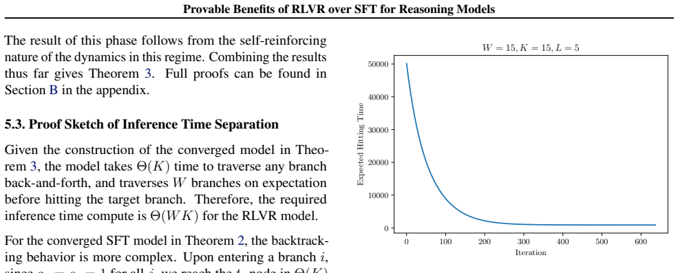
When exiting the branch, starting from the stateR + K+1 (i.e. reached the state with headt i), letg i denote the expected time of first entry into R− K+1−i, and fi denote the expected time of first entry into L− K+1−i. Then, with the base case ofg 1 = 1, we have the following recursion: fi = L+ 1 L gi + (2i−1)· 1 L + 1, gi = (L+ 1)f i−1 + (2i−2)·L+ 1. Hen...

2000

[1] [1]

Scaling LLM Test-Time Compute Optimally can be More Effective than Scaling Model Parameters

URL https://openreview.net/forum? id=hJ2BCYGvFg. Snell, C., Lee, J., Xu, K., and Kumar, A. Scaling LLM test- time compute optimally can be more effective than scal- ing model parameters.arXiv preprint arXiv:2408.03314, 2024. Sutton, R. S., McAllester, D., Singh, S., and Mansour, Y . Policy gradient methods for reinforcement learning with function approxim...

work page internal anchor Pith review Pith/arXiv arXiv 2024

[2] [2]

Reinforcement Learning for Reasoning in Large Language Models with One Training Example

URL https://proceedings.neurips. cc/paper_files/paper/1999/file/ 464d828b85b0bed98e80ade0a5c43b0f-Paper. pdf. Wang, Y ., Yang, Q., Zeng, Z., Ren, L., Liu, L., Peng, B., Cheng, H., He, X., Wang, K., Gao, J., Chen, W., Wang, S., Du, S. S., and Shen, Y . Reinforcement learning for reasoning in large language models with one training example, 2025. URL https:...

work page internal anchor Pith review Pith/arXiv arXiv 1999

[3] [3]

Let Hf :=h x(ui,1,l →f) denote the hitting time of a fixed target x from any of the states whose head is the fork f (including the initial source states 0 →f); by symmetry they are all equal, hence why we consider a single value

[4] [4]

That is, ˜g(s) :=E[τf] where τf := min{t≥0 :s 0 =s,head(s t) =f}

For state s not on the branch of x, we define ˜g(s)to be the expected time of hitting the fork, starting at state s. That is, ˜g(s) :=E[τf] where τf := min{t≥0 :s 0 =s,head(s t) =f} . In particular, this means that hx(s) = ˜g(s) +Hf , and we have the absorbing conditionh x(ui,1,l →f) = 0for branchinot equal to the branch of targetx. 17 Provable Benefits o...

[5] [5]

both states are absorbing)

For state s on the branch of x, we define g(s) to be the expected time of hitting either f or x (e.g. both states are absorbing). That is,g(s) :=E[τ {f,x}]whereτ {f,x} := min{t≥0 :s 0 =s,head∈ {f, x}}

[6] [6]

In particular, this means that hx(s) =g(s) +q(s)H f

For state s on the branch of x, we define q(s) to be the probability it hits f before x. In particular, this means that hx(s) =g(s) +q(s)H f . Lemma 7.Define the followingq-gaps: δj :=q(L − j )−q(L + j+1), ϵ j :=q(R − j−1)−q(R + j ) Then, it holds thatδ j >0andϵ j >0for allj. Proof. For δj, this follows intuitively from the fact that all paths from L+ j+1...

[7] [7]

In other words, µs is the expected number of visits to statesduring a target branch attempt

When s is on the target branch, define µ(s) :=E hP t<τ{f,x} 1{st =s}|s 0 =L + 1 i . In other words, µs is the expected number of visits to statesduring a target branch attempt

[8] [8]

In other words, ˜µs is the expected number of visits to statesduring a non-target branch attempt until it goes back tof

When s is not on the target branch, define ˜µ(s) :=E hP t<τf 1{st =s}|s 0 =L + 1 i . In other words, ˜µs is the expected number of visits to statesduring a non-target branch attempt until it goes back tof. Definition 3.Fix a target x, and define the success probability of hitting the target upon entering its branchpsucc before hittingf. That is, psucc :=P...

[9] [9]

Ifsis on the same branch asx, then we haved x(s) = µ(s) psucc

[10] [10]

Ifsis on a different branch fromx, then we haved x(s) = ˜µ(s) psucc . Proof. Note that the probability of success for each branch entry is psucc W , as one needs to choose the target branch with probability 1/W and then succeed with probability psucc. Hence, the total number of fork departures on expectation is W/psucc, so the expected number of entries i...

[11] [11]

On a non-target branch, it holds thatd x(L+ j ) =d x(R− j ) =Dandd x(R+ j ) =d x(L− j ) =D·L

[12] [12]

The hitting time from a fork state isH 0 :=H f(0) = (2W−1)D(1 +K(L+ 1)). 26 Provable Benefits of RLVR over SFT for Reasoning Models On a non-target branch, it holds at initialization (t= 0 ) that ˜µ(s) = 1for non-multiedge states and ˜µ(s) =Lfor aggregate multiedge states. That is,˜µ(L+ j ) = ˜µ(R− j ) = 1and˜µ(L− j ) = ˜µ(R+ j ) =L. For all1≤j≤K, it hold...

[13] [13]

Upon entering a branchi, sincea j =c j = 1for allj, we reach thet i node inΘ(K)time

[14] [14]

reached the state with headt i), letg i denote the expected time of first entry into R− K+1−i, and fi denote the expected time of first entry into L− K+1−i

When exiting the branch, starting from the stateR + K+1 (i.e. reached the state with headt i), letg i denote the expected time of first entry into R− K+1−i, and fi denote the expected time of first entry into L− K+1−i. Then, with the base case ofg 1 = 1, we have the following recursion: fi = L+ 1 L gi + (2i−1)· 1 L + 1, gi = (L+ 1)f i−1 + (2i−2)·L+ 1. Hen...

2000