A thorough investigation of cross-correlation estimators for stochastic gravitational-wave background searches in ground-based detector data
Pith reviewed 2026-06-26 07:14 UTC · model grok-4.3
The pith
Reformulating cross-correlation estimators in the frequency domain for stochastic gravitational-wave background searches yields new narrowband expressions whose covariances differ from prior usage, yet the older expressions produce correct
A machine-rendered reading of the paper's core claim, the machinery that carries it, and where it could break.
Core claim
The central claim is that a frequency-domain reformulation of the cross-correlation method resolves issues with covariances induced by time-domain windowing and overlapping, producing new expressions for narrowband estimators, but that the previously used expressions nevertheless yield correct posterior distributions for parameter estimation and correct log-Bayes factors for model selection.
What carries the argument
The frequency-domain narrowband cross-correlation estimators, with explicit accounting for covariances from windowing and overlapping of data segments.
If this is right
- Analyses can now use narrowband estimators with a robust theoretical foundation for characterizing the energy density in specific frequency bins.
- More accurate and physically insightful interpretations of stochastic gravitational-wave background observations become possible.
- The framework lays a foundation for current and future research in stochastic gravitational-wave background searches.
- Parameter estimation and model selection remain reliable even when using the previously standard expressions.
Where Pith is reading between the lines
- The validation of old expressions suggests that past searches for stochastic backgrounds may not need re-analysis for their inference results.
- Future work could test the new expressions on simulated data to quantify any practical differences in narrowband cases.
- Similar reformulations might apply to other signal searches that use cross-correlations in ground-based detectors.
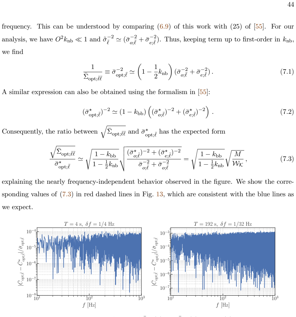
Load-bearing premise
That the non-zero covariances induced by windowing and overlapping of data in the time domain are the main unresolved issue when formulating narrowband estimators in the frequency domain.
What would settle it
A direct comparison on real or simulated detector data showing whether posterior distributions or log-Bayes factors differ when using the new versus old covariance expressions for narrowband estimators.
Figures


read the original abstract
Detecting a stochastic gravitational-wave background represents a crucial yet challenging objective within the field of gravitational-wave astronomy. Ground-based detectors currently rely almost exclusively on cross-correlation methods to detect stochastic gravitational-wave background signals. Traditionally, these methods define and optimize a broadband estimator initially constructed in the time domain. However, a growing number of analyses require precise narrowband estimators to accurately characterize the energy density of the underlying signal in specific frequency bins. Transitioning from time-domain broadband estimators to frequency-domain narrowband estimators introduces significant complexities that have not yet been fully explored in the existing literature. In this study, we systematically revisit and rigorously reformulate the cross-correlation method in the frequency domain, explicitly addressing and resolving issues related to non-zero covariances induced by windowing and overlapping of data in the time domain. We provide new expressions for the narrowband estimators and their covariances, which differ from those used in past searches. Fortunately, we show that the expressions that have been widely used in the field nonetheless lead to correct posterior distributions for parameter estimation and correct log-Bayes factors for model selection. By establishing a robust theoretical framework, our work facilitates more accurate and physically insightful interpretations of stochastic gravitational-wave background observations, laying an essential foundation for current and future research in this field.
Editorial analysis
A structured set of objections, weighed in public.
Referee Report
Summary. The manuscript reformulates the cross-correlation method for stochastic gravitational-wave background (SGWB) searches from the time domain to the frequency domain. It derives new expressions for narrowband estimators and their covariances that explicitly resolve non-zero covariances induced by windowing and overlapping of data segments. These new expressions differ from those used in past searches, but the authors demonstrate that the legacy expressions nonetheless produce correct posterior distributions for parameter estimation and correct log-Bayes factors for model selection.
Significance. If the central derivations and equivalence demonstrations hold, the work is significant for SGWB analyses in LIGO/Virgo/KAGRA data. It supplies a rigorous frequency-domain framework that clarifies why existing narrowband pipelines remain valid for inference while enabling more precise physical interpretations of energy-density spectra. The explicit validation of legacy methods for posteriors and Bayes factors strengthens confidence in published results without requiring reanalysis of existing datasets.
minor comments (3)
- [§3] §3 (or equivalent derivation section): the transition from the time-domain broadband estimator to the frequency-domain narrowband form would benefit from an explicit side-by-side comparison table of the legacy versus new covariance expressions to make the differences immediately visible to readers.
- [Figure 2] Figure 2 (or the figure showing covariance matrices): axis labels and color-bar scaling should be clarified so that the off-diagonal terms induced by overlap are quantitatively readable without reference to the text.
- [§5] The statement that the legacy expressions 'lead to correct posterior distributions' would be strengthened by a brief remark on the precise sense in which 'correct' is defined (e.g., identical to the new expressions up to a normalization factor that cancels in the likelihood ratio).
Simulated Author's Rebuttal
We thank the referee for their positive and accurate summary of our manuscript, as well as for recommending acceptance. The referee correctly identifies the central result: new frequency-domain expressions for narrowband estimators and covariances, together with the demonstration that legacy expressions remain valid for posterior inference and model selection.
Circularity Check
No significant circularity
full rationale
The paper performs a direct mathematical reformulation of time-domain broadband cross-correlation estimators into frequency-domain narrowband estimators, explicitly deriving new expressions for the estimators and their covariances to account for windowing-induced correlations. It then demonstrates that the legacy expressions remain valid for posterior inference and Bayes factors. No load-bearing step reduces by construction to a fitted parameter, self-citation chain, or definitional equivalence; the central results are independent derivations from the underlying time-domain statistics. The work is self-contained against external benchmarks with no circular reduction exhibited.
Axiom & Free-Parameter Ledger
axioms (1)
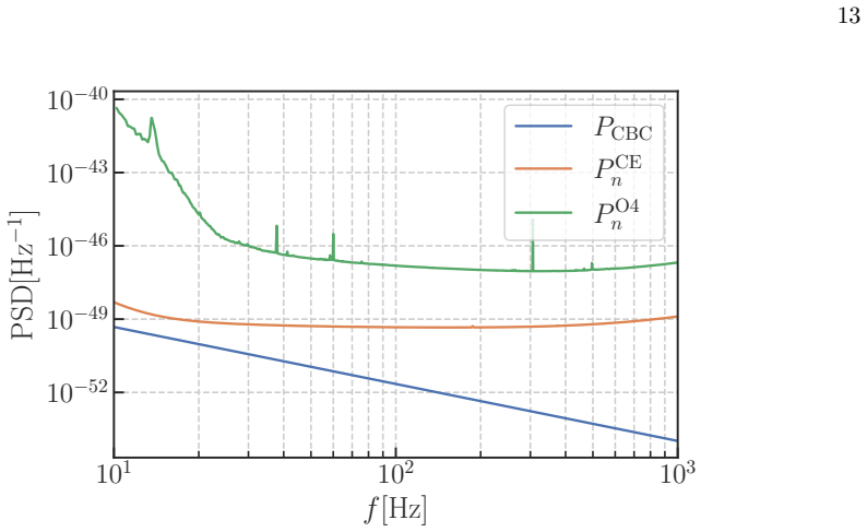
- domain assumption Detector noise is stationary and Gaussian with known power spectral densities
Reference graph
Works this paper leans on
-
[1]
Single-component SGWB: In this case, we assume that there is only one source of the SGWB, so that we can always express Ωgw(f |θ) by the product of a single amplitude Ω s and frequency-dependent function F (f |θ−): Ωgw(f) = ΩsF (f |θ−), (8.8) 48 where θ ≡ {Ωs} ⊕ θ−, with θ− ≡ {θ1, θ2, ...} encapsulating all the remaining model param- eters. Given this par...
-
[2]
In this case, the definition of R¯ℓ requires all parameters θ = {Ωs;i}Ns i=1 ⊕ {θ− i }Ns i=1
Multi-component SGWB: If we assume there are multiple sources contributing to Ω gw(f), then we can parametrize Ωgw(f) as follows: Ωgw(f) = NsX i=1 Ωs;iFi(f |θ− i ), (8.9) where Ω s;i and Fi(fi|θ− i ) describe the amplitude and frequency-dependence of Ω gw(f) for the ith source model, respectively. In this case, the definition of R¯ℓ requires all parameter...
-
[4]
F. Acernese et al. (VIRGO), Class. Quant. Grav. 32, 024001 (2015), arXiv:1408.3978 [gr-qc]
Pith/arXiv arXiv 2015
-
[5]
D. Bersanetti, B. Patricelli, O. J. Piccinni, F. Piergiovanni, F. Salemi, and V. Sequino, Universe 7 (2021), 10.3390/universe7090322. 57
-
[6]
T. Akutsu et al. (KAGRA), Nature Astron. 3, 35 (2019), arXiv:1811.08079 [gr-qc]
arXiv 2019
-
[7]
R. Abbott et al. (KAGRA, VIRGO, LIGO Scientific), Phys. Rev. X13, 011048 (2023), arXiv:2111.03634 [astro-ph.HE]
Pith/arXiv arXiv 2023
-
[8]
R. Abbott et al. (KAGRA, Virgo, LIGO Scientific), Phys. Rev. D104, 022004 (2021), arXiv:2101.12130 [gr-qc]
arXiv 2021
-
[9]
A. I. Renzini, B. Goncharov, A. C. Jenkins, and P. M. Meyers, Galaxies 10, 34 (2022), arXiv:2202.00178 [gr-qc]
arXiv 2022
-
[10]
Abbott et al
R. Abbott et al. (LIGO Scientific Collaboration, Virgo Collaboration, and KAGRA Collaboration), Phys. Rev. D 104, 022004 (2021)
2021
-
[11]
D. S. Bellie, S. Banagiri, Z. Doctor, and V. Kalogera, Phys. Rev. D 110, 023006 (2024), arXiv:2310.02517 [gr-qc]
arXiv 2024
-
[12]
Kosowsky, M
A. Kosowsky, M. S. Turner, and R. Watkins, Phys. Rev. D 45, 4514 (1992)
1992
-
[13]
Kosowsky and M
A. Kosowsky and M. S. Turner, Phys. Rev. D 47, 4372 (1993)
1993
-
[14]
P. S. B. Dev and A. Mazumdar, Phys. Rev. D 93, 104001 (2016)
2016
-
[15]
Marzola, A
L. Marzola, A. Racioppi, and V. Vaskonen, The European Physical Journal C 77, 484 (2017)
2017
-
[16]
von Harling, A
B. von Harling, A. Pomarol, O. Pujol` as, and F. Rompineve, Journal of High Energy Physics 2020, 195 (2020)
2020
- [17]
-
[18]
R. Jinno and M. Takimoto, Phys. Rev. D 95, 024009 (2017), arXiv:1605.01403 [astro-ph.CO]
Pith/arXiv arXiv 2017
-
[19]
V. Ferrari, S. Matarrese, and R. Schneider, Mon. Not. Roy. Astron. Soc. 303, 247 (1999), arXiv:astro- ph/9804259
arXiv 1999
-
[20]
A. Buonanno, G. Sigl, G. G. Raffelt, H.-T. Janka, and E. Muller, Phys. Rev. D 72, 084001 (2005), arXiv:astro-ph/0412277
Pith/arXiv arXiv 2005
-
[21]
K. Crocker, V. Mandic, T. Regimbau, K. Belczynski, W. Gladysz, K. Olive, T. Prestegard, and E. Vangioni, Phys. Rev. D 92, 063005 (2015), arXiv:1506.02631 [gr-qc]
Pith/arXiv arXiv 2015
-
[22]
K. Crocker, T. Prestegard, V. Mandic, T. Regimbau, K. Olive, and E. Vangioni, Phys. Rev. D 95, 063015 (2017), arXiv:1701.02638 [astro-ph.CO]
Pith/arXiv arXiv 2017
- [23]
-
[24]
L. P. Grishchuk, Zh. Eksp. Teor. Fiz. 67, 825 (1974)
1974
-
[25]
A. A. Starobinsky, JETP Lett. 30, 682 (1979)
1979
-
[26]
L. P. Grishchuk, Phys. Rev. D 48, 3513 (1993), arXiv:gr-qc/9304018
Pith/arXiv arXiv 1993
-
[27]
N. Barnaby, E. Pajer, and M. Peloso, Phys. Rev. D 85, 023525 (2012), arXiv:1110.3327 [astro-ph.CO]
Pith/arXiv arXiv 2012
-
[28]
T. Damour and A. Vilenkin, Phys. Rev. D 71, 063510 (2005), arXiv:hep-th/0410222
Pith/arXiv arXiv 2005
-
[29]
X. Siemens, V. Mandic, and J. Creighton, Phys. Rev. Lett. 98, 111101 (2007), arXiv:astro-ph/0610920
Pith/arXiv arXiv 2007
-
[30]
S. Olmez, V. Mandic, and X. Siemens, Phys. Rev. D 81, 104028 (2010), arXiv:1004.0890 [astro-ph.CO]
Pith/arXiv arXiv 2010
-
[31]
T. Regimbau, S. Giampanis, X. Siemens, and V. Mandic, Phys. Rev. D 85, 066001 (2012), arXiv:1111.6638 [astro-ph.CO]. 58
Pith/arXiv arXiv 2012
-
[32]
R. Abbott et al. (LIGO Scientific, Virgo), Astrophys. J. Lett. 913, L7 (2021), arXiv:2010.14533 [astro- ph.HE]
arXiv 2021
-
[33]
S. S. Bavera, G. Franciolini, G. Cusin, A. Riotto, M. Zevin, and T. Fragos, Astron. Astrophys. 660, A26 (2022), arXiv:2109.05836 [astro-ph.CO]
arXiv 2022
-
[34]
D. Reitze, R. X. Adhikari, S. Ballmer, B. Barish, L. Barsotti, G. Billingsley, D. A. Brown, Y. Chen, D. Coyne, R. Eisenstein, et al., arXiv:1907.04833 (2019)
Pith/arXiv arXiv 1907
-
[35]
Punturo, M
M. Punturo, M. Abernathy, F. Acernese, et al., Classical and Quantum Gravity 27, 194002 (2010)
2010
-
[36]
S. Drasco and E. E. Flanagan, Phys. Rev. D 67, 082003 (2003), arXiv:gr-qc/0210032
Pith/arXiv arXiv 2003
-
[37]
R. Smith and E. Thrane, Phys. Rev. X 8, 021019 (2018), arXiv:1712.00688 [gr-qc]
Pith/arXiv arXiv 2018
-
[38]
R. J. E. Smith, C. Talbot, F. Hernandez Vivanco, and E. Thrane, Mon. Not. Roy. Astron. Soc. 496, 3281 (2020), arXiv:2004.09700 [astro-ph.HE]
arXiv 2020
-
[39]
Biscoveanu, C
S. Biscoveanu, C. Talbot, E. Thrane, and R. Smith, Phys. Rev. Lett. 125, 241101 (2020)
2020
-
[40]
J. Lawrence, K. Turbang, A. Matas, A. I. Renzini, N. van Remortel, and J. D. Romano, Phys. Rev. D 107, 103026 (2023), arXiv:2301.07675 [gr-qc]
arXiv 2023
-
[41]
B. Allen and J. D. Romano, Phys. Rev. D 59, 102001 (1999), arXiv:gr-qc/9710117
Pith/arXiv arXiv 1999
-
[42]
J. D. Romano and N. J. Cornish, Living Rev. Rel. 20, 2 (2017), arXiv:1608.06889 [gr-qc]
Pith/arXiv arXiv 2017
-
[43]
V. Mandic, E. Thrane, S. Giampanis, and T. Regimbau, Phys. Rev. Lett. 109, 171102 (2012), arXiv:1209.3847 [astro-ph.CO]
Pith/arXiv arXiv 2012
-
[44]
Lazzarini and J
A. Lazzarini and J. Romano, Use of Overlapping Windows in the Stochastic Background Search, LIGO Technical Note LIGO-T040089-00-Z (LIGO Laboratory, 2004) LIGO Document T040089-00. https://dcc.ligo.org/T040089/public
2004
-
[45]
J. T. Whelan, Cross-correlation of windowed, discretely-sampled data, LIGO Technical Note LIGO- T040125-00-Z (LIGO Laboratory, 2004) LIGO Document T040125-00. https://dcc.ligo.org/ LIGO-T040125/public
2004
-
[46]
Sundaresan and J
S. Sundaresan and J. T. Whelan, Windowing and Leakage in the Cross-Correlation Search for Periodic Gravitational Waves, LIGO Technical Note LIGO-T1200431-v1 (LIGO Laboratory, 2012) LIGO Document T1200431-v1. https://dcc.ligo.org/LIGO-T1200431-v1/public
2012
-
[47]
J. T. Whelan, S. Sundaresan, Y. Zhang, and P. Peiris, Phys. Rev. D 91, 102005 (2015)
2015
- [48]
-
[49]
A. I. Renzini, T. Callister, K. Chatziioannou, and W. M. Farr, Phys. Rev. D 110, 023014 (2024), arXiv:2403.14793 [astro-ph.HE]
arXiv 2024
-
[50]
B. Cousins, K. Schumacher, A. K.-W. Chung, C. Talbot, T. Callister, D. E. Holz, and N. Yunes, arXiv (2025), arXiv:2503.01997 [astro-ph.CO]
arXiv 2025
-
[51]
T. Callister, M. Fishbach, D. Holz, and W. Farr, Astrophys. J. Lett. 896, L32 (2020), arXiv:2003.12152 [astro-ph.HE]
arXiv 2020
-
[52]
T. Callister, L. Jenks, D. E. Holz, and N. Yunes, Phys. Rev. D 111, 044041 (2025), arXiv:2312.12532 [gr-qc]. 59
arXiv 2025
-
[53]
K. Turbang, M. Lalleman, T. A. Callister, and N. van Remortel, Astrophys. J. 967, 142 (2024), arXiv:2310.17625 [astro-ph.HE]
arXiv 2024
-
[54]
S. W. Ballmer, Class. Quant. Grav. 23, S179 (2006), gr-qc/0510096
Pith/arXiv arXiv 2006
-
[55]
Dhurandhar, B
S. Dhurandhar, B. Krishnan, H. Mukhopadhyay, and J. T. Whelan, Phys. Rev. D 77, 082001 (2008)
2008
-
[56]
A. Matas and J. D. Romano, Phys. Rev. D 103, 062003 (2021), arXiv:2012.00907 [gr-qc]
arXiv 2021
-
[57]
A. I. Renzini et al., Astrophys. J. 952, 25 (2023), arXiv:2303.15696 [gr-qc]
arXiv 2023
-
[58]
C. M. F. Mingarelli, S. R. Taylor, B. S. Sathyaprakash, and W. M. Farr, arXiv preprint (2019), arXiv:1911.09745 [gr-qc]
arXiv 2019
-
[59]
Allen and J
B. Allen and J. D. Romano, Phys. Rev. Lett. 134, 031401 (2025)
2025
-
[60]
Noise curves for use in simulations pre-O4,
LIGO Scientific Collaboration, Virgo Collaboration, and KAGRA Collaboration, “Noise curves for use in simulations pre-O4,” LIGO Document Control Center, LIGO-T2200043-v3 (2022), https://dcc. ligo.org/T2200043-v3/public
2022
-
[61]
V. Srivastava, D. Davis, K. Kuns, P. Landry, S. Ballmer, M. Evans, E. D. Hall, J. Read, and B. S. Sathyaprakash, Astrophys. J. 931, 22 (2022), arXiv:2201.10668 [gr-qc]
arXiv 2022
-
[62]
A. G. Abac et al. (LIGO Scientific, VIRGO, KAGRA), (2025), arXiv:2508.20721 [gr-qc]
arXiv 2025
-
[63]
R. Caldwell et al., Gen. Rel. Grav. 54, 156 (2022), arXiv:2203.07972 [gr-qc]
arXiv 2022
-
[64]
D. Phan, N. Pradhan, and M. Jankowiak, arXiv preprint arXiv:1912.11554 (2019)
Pith/arXiv arXiv 1912
-
[65]
Bingham, J
E. Bingham, J. P. Chen, M. Jankowiak, F. Obermeyer, N. Pradhan, T. Karaletsos, R. Singh, P. A. Szerlip, P. Horsfall, and N. D. Goodman, J. Mach. Learn. Res. 20, 28:1 (2019)
2019
-
[66]
Wick’s Theorem
L. Isserlis, Biometrika 12, 134 (1918), often called “Wick’s Theorem” by physicists, although Wick’s work was three decades later
1918
-
[67]
P. D. Welch, IEEE Transactions on Audio and Electroacoustics 15, 70 (1967)
1967
-
[68]
W. H. Press, S. A. Teukolsky, W. T. Vetterling, and B. P. Flannery, Numerical Recipes: The Art of Scientific Computing, 3rd ed. (Cambridge University Press, USA, 2007)
2007
-
[69]
G. M. Harry (LIGO Scientific), Class. Quant. Grav. 27, 084006 (2010)
2010
-
[70]
J. Aasi et al. (LIGO Scientific), Class. Quant. Grav. 32, 074001 (2015), arXiv:1411.4547 [gr-qc]
Pith/arXiv arXiv 2015
-
[71]
G. Ashton et al., Astrophys. J. Suppl. 241, 27 (2019), arXiv:1811.02042 [astro-ph.IM]
Pith/arXiv arXiv 2019
-
[72]
Ashton, M
G. Ashton, M. H¨ ubner, P. D. Lasky, C. Talbot, K. Ackley, S. Biscoveanu, Q. Chu, A. Divakarla, P. J. Easter, B. Goncharov, et al., The Astrophysical Journal Supplement Series 241, 27 (2019). Appendix A: Statistics: standard definitions and results In this appendix, we review some standard definitions and results in statistics, which we will use repeatedl...
2019
-
[73]
Its mean (expected value) and variance are defined as follows: µx ≡ ⟨x⟩ ≡ Z dx p(x)x , (A.1) σ2 x ≡ ⟨x2⟩ − ⟨x⟩2
Mean, variance, and covariance Consider a random variable x. Its mean (expected value) and variance are defined as follows: µx ≡ ⟨x⟩ ≡ Z dx p(x)x , (A.1) σ2 x ≡ ⟨x2⟩ − ⟨x⟩2 . (A.2) Now, suppose we have N (real) random variables x1, x 2, · · · , x N. Their mutual dependence can be quantified by their covariance, defined as Σij ≡ ⟨xixj⟩ − ⟨xi⟩⟨xj⟩ . (A.3) I...
-
[74]
Isserlis’s theorem Consider N zero-mean, Gaussian random variables x1, x 2, · · · , xN. According to Isserlis’s theorem [64], the Nth-order expectation value can be written as ⟨x1x2 · · · xN ⟩ = X p∈P 2 N Y {i,j}∈p ⟨xixj⟩ , (A.5) where p denotes all possible distinct ways of partitioning {1, 2, · · · , N} into pairs (i, j). The sum- mation above is over a...
-
[75]
Suppose now that they all have the same mean ⟨xi⟩ = a, ∀xi, and the covariance Σ ij is known
Optimal estimator Consider again N random variables x1, x 2, · · · , xN. Suppose now that they all have the same mean ⟨xi⟩ = a, ∀xi, and the covariance Σ ij is known. Then we can construct a linear optimal estimator of a such that the estimator is unbiased and has the minimum variance. We define the optimal estimator ˆaopt by the linear combination ˆaopt ...
-
[76]
Consider N Gaussian-distributed random variables, xi = a + ni , i = 1, 2, · · · , N, (A.13) with ⟨ni⟩ = 0, ⟨ninj⟩ = σ2δij
Sufficient statistics We introduce the idea of sufficient statistics by considering the following toy example, and refer the interested readers to [54] for extra discussion. Consider N Gaussian-distributed random variables, xi = a + ni , i = 1, 2, · · · , N, (A.13) with ⟨ni⟩ = 0, ⟨ninj⟩ = σ2δij . (A.14) In the above expressions, a denotes the unknown ampl...
-
[77]
(4.5) We want to evaluate the summation Sℓ ≡PN −1 j=0 ˜wℓ−j ˜w∗ ℓ−j
Proof of Eq. (4.5) We want to evaluate the summation Sℓ ≡PN −1 j=0 ˜wℓ−j ˜w∗ ℓ−j. Using the definition the DFT (2.5), we find Sℓ = (∆t)2 N −1X j=0 N −1X p=0 N −1X q=0 wpwqe−2πi p(ℓ−j) N e2πi q(ℓ−j) N = (∆t)2 N −1X p=0 N −1X q=0 wpwqe−2πi ℓ(p−q) N N −1X j=0 e2πi j(p−q) N | {z } N δpq . (B.1) Note that the summation over j yields a Kronecker delta, δpq, whi...
-
[78]
(4.11) We now want to evaluate Spq ≡PN −1 j=0 ˜wp−j ˜w∗ q−j
Proof of Eq. (4.11) We now want to evaluate Spq ≡PN −1 j=0 ˜wp−j ˜w∗ q−j. As before, we use the definition of the DFT (Eq. (2.5)) to obtain: Spq = (∆t)2 N −1X j=0 N −1X ℓ=0 N −1X m=0 wℓwme−2πi ℓ(p−j) N e2πi m(q−j) N = (∆t)2 N −1X ℓ=0 N −1X m=0 wℓwme−2πi (ℓp−mq) N N −1X j=0 e2πi j(ℓ−m) N | {z } N δℓm = T 2 N N −1X ℓ=0 w2 ℓ e−2πi ℓ(p−q) N . (B.3) 64
-
[79]
(4.22) To prove (4.22), we need to evaluate S − jk;¯ℓ ¯m and S+ jk;¯ℓ; ¯m defined in (4.21)
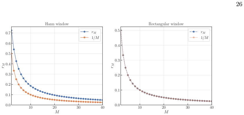
Proof of Eq. (4.22) To prove (4.22), we need to evaluate S − jk;¯ℓ ¯m and S+ jk;¯ℓ; ¯m defined in (4.21). Let us first consider S − jk;¯ℓ ¯m: S − jk;¯ℓ ¯m ≡ 1 M 2 M ¯ℓ+ M 2 −1X p=M ¯ℓ− M 2 M ¯m+ M 2 −1X q=M ¯m− M 2 e−2πi(j−k) (p−q) N = e−2πi(j−k) M(¯ℓ− ¯m) N 1 M 2 M −1X p,q=0 e−2πi(j−k) (p−q) N = e−2πi(j−k) M(¯ℓ− ¯m) N 1 M M −1X p=0 e−2πi(j−k) p N 2 . (B....
-
[80]
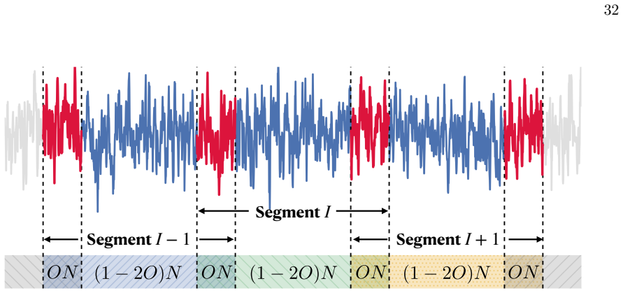
Proof of Eq. (5.7) We start by proving (5.7), which we can be derived from (5.5) as follows: ⟨ ˜d1;I;j ˜d∗ 1;I+1;k⟩ = (∆t)2 N −1X r=0 N −1X s=0 ⟨d1;I;rd1;I+1;s⟩e−2πi rj N e2πi sk N e2πi (1−O)N k N = (∆t)2 N −1X r=0 (2−O)N −1X s=(1−O)N ⟨dI+ 1;rdI+ 1;s⟩e−2πi rj N e2πi [s−(1−O)N]k N e2πi (1−O)N k N = (∆t)2 N −1X r=0 (2−O)N −1X s=(1−O)N ⟨dI+ 1;rdI+ 1;s⟩e−2πi ...
-
[81]
(5.8) To prove (5.8), we continue with the last equality of (C.1), noting that⟨dI+ 1;rdI+ 1;s⟩ is the definition of the auto-correlation function σ2 1R1;|r−s| for detector 1
Proof of Eq. (5.8) To prove (5.8), we continue with the last equality of (C.1), noting that⟨dI+ 1;rdI+ 1;s⟩ is the definition of the auto-correlation function σ2 1R1;|r−s| for detector 1. Then, ⟨ ˜d1;I;j ˜d∗ 1;I+1;k⟩ = (∆t)2 N −1X r=0 (2−O)N −1X s=(1−O)N σ2 1R1;|r−s|e−2πi (rj−sk) N = (∆t)2 N −1X r=0 min r+N −1,(2−O)N −1 X s=(1−O)N σ2 1R1;|r−s|e−2πi (rj−sk...
discussion (0)
Sign in with ORCID, Apple, or X to comment. Anyone can read and Pith papers without signing in.